Author: Gabriel Rüeck
Setting up Client VPNs, Policy Routing
Executive Summary
This blog post is the continuation my previous blog post Setting up Dual Stack VPNs and explains how I use client VPNs together with simple Policy Routing on my Linux server in order to relegate outgoing connections to various network interfaces and, ultimately, to different countries. The examples use IPv4 only.
Background
The approach was originally developed back in 2011…2014 when I lived in China and maintained several outgoing VPN connections from my Linux server to end points “in the West” so that I could circumvent internet censorship in China [8]. With the VPN service described Setting up Dual Stack VPNs, it was then possible for me to be in town and to connect the smartphone to my Linux server (in the same town). From there, the connections to sites blocked in China would run over the client VPNs of the Linux server so that I could use Google Maps on my smartphone, for example (which at that time had already been blocked in China).
Preconditions
Routing in Linux follows some very clever approaches which can be combined in mighty ways. Those readers who want to understand all of the underlying theory, are encouraged to study the (older) documents [1], [2], [3], even if parts of the content might not be relevant any more. Those readers who just want to follow and replicate the approach in this blog, should at least study the documents [4], [5], [6].
Apart from that, in order to replicate the approach described here, you should:
- … fulfil all preconditions listed in the blog post Setting up Dual Stack VPNs
- … have running the setup similar to the one described in the blog post Setting up Dual Stack VPNs
- … have access to a commercial VPN provider allowing you to run several client connections on the same machine
- … have at least read the documents [4], [5], [6]
Description and Usage
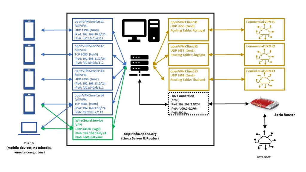
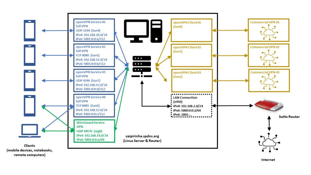
The graph below shows the setup on my machine caipirinha.spdns.org with. The 5 VPN services (blue, green color) were already described in blog post Setting up Dual Stack VPNs. Now, we have a close look at the 3 VPN clients which use a commercial VPN service (ocker color) in order to connect to VPN end points in 3 different countries (Portugal, Singapore, Thailand).
Enabling Routing
Routing needs to be enabled on the Linux server. I personally also decided to switch off the privacy extensions on the Linux server, but that is a personal matter of taste:
# Enable "loose" reverse path filtering and prohibit icmp redirects
sysctl -w net.ipv4.conf.all.rp_filter=2
sysctl -w net.ipv4.conf.all.send_redirects=0
sysctl -w net.ipv4.conf.eth0.send_redirects=0
sysctl -w net.ipv4.icmp_errors_use_inbound_ifaddr=1

# Enable IPv6 routing, but keep SLAAC for eth0
sysctl -w net.ipv6.conf.eth0.accept_ra=2
sysctl -w net.ipv6.conf.all.forwarding=1

# Switch off the privacy extensions
sysctl -w net.ipv6.conf.eth0.use_tempaddr=0
Routing Tables
We now must have a closer look at the concept of the routing table. A routing tables basically lists routes to particular network destinations. An example is the routing table main on my Linux server. It reads:
caipirinha:~ # ip route list table main
default via 192.168.2.1 dev eth0 proto dhcp
192.168.2.0/24 dev eth0 proto kernel scope link src 192.168.2.3
192.168.10.0/24 dev tun4 proto kernel scope link src 192.168.10.1
192.168.11.0/24 dev tun5 proto kernel scope link src 192.168.11.1
192.168.12.0/24 dev tun6 proto kernel scope link src 192.168.12.1
192.168.13.0/24 dev tun7 proto kernel scope link src 192.168.13.1
192.168.14.0/24 dev wg0 proto kernel scope link src 192.168.14.1
This table has 7 entries, and they have this meaning:
- (“default via…”) Connections to IP addresses that do not have a corresponding entry in the routing table shall be forwarded via the interface eth0 and to the router IP address 192.168.2.1 (an AVM Fritz! Box).
- Connections to the network 192.168.2.0/24 shall be forwarded via the interface eth0 using the source IP address 192.168.2.3 (the Linux server itself).
- Connections to the network 192.168.10.0/24 shall be forwarded via the interface tun4 using the source IP address 192.168.10.1 (the Linux server itself). This network belongs to one of the 5 VPN services on my Linux server.
- Connections to the network 192.168.11.0/24 shall be forwarded via the interface tun5 using the source IP address 192.168.11.1 (the Linux server itself). This network belongs to one of the 5 VPN services on my Linux server.
- Connections to the network 192.168.12.0/24 shall be forwarded via the interface tun6 using the source IP address 192.168.12.1 (the Linux server itself). This network belongs to one of the 5 VPN services on my Linux server.
- Connections to the network 192.168.13.0/24 shall be forwarded via the interface tun7 using the source IP address 192.168.13.1 (the Linux server itself). This network belongs to one of the 5 VPN services on my Linux server.
- Connections to the network 192.168.14.0/24 shall be forwarded via the interface wg0 using the source IP address 192.168.14.1 (the Linux server itself). This network belongs to one of the 5 VPN services on my Linux server.
Usually, a routing table should have a default entry which sends all IP traffic that is not explicitly routed to other network interfaces to the default router of a network. Otherwise, no meaningful internet access is possible.
A Linux system can have up to 256 routing tables which are defined in /etc/iproute2/rt_tables. They can either be used by their number or by their name. On my Linux server, I have set up 3 additional routing tables, named “Portugal”, “Singapur”, “Thailand”. You can see in the file /etc/iproute2/rt_tables that besides the table main, the tables local, default, and unspec do already exist, but they are not of interest for our purposes.
#
# reserved values
#
255 local
254 main
253 default
0 unspec
#
# local
#
#1  inr.ruhep

240 Portugal
241 Singapur
242 Thailand
Right now (before we set up the client VPNs), all 3 routing tables look the same as shown here:
caipirinha:~ # ip route list table Portugal
192.168.2.0/24 dev eth0 proto kernel scope link src 192.168.2.3
192.168.10.0/24 via 192.168.10.1 dev tun4
192.168.11.0/24 via 192.168.11.1 dev tun5
192.168.12.0/24 via 192.168.12.1 dev tun6
192.168.13.0/24 via 192.168.13.1 dev tun7
192.168.14.0/24 via 192.168.14.1 dev wg0
caipirinha:~ # ip route list table Singapur
192.168.2.0/24 dev eth0 proto kernel scope link src 192.168.2.3
192.168.10.0/24 via 192.168.10.1 dev tun4
192.168.11.0/24 via 192.168.11.1 dev tun5
192.168.12.0/24 via 192.168.12.1 dev tun6
192.168.13.0/24 via 192.168.13.1 dev tun7
192.168.14.0/24 via 192.168.14.1 dev wg0
caipirinha:~ # ip route list table Thailand
192.168.2.0/24 dev eth0 proto kernel scope link src 192.168.2.3
192.168.10.0/24 via 192.168.10.1 dev tun4
192.168.11.0/24 via 192.168.11.1 dev tun5
192.168.12.0/24 via 192.168.12.1 dev tun6
192.168.13.0/24 via 192.168.13.1 dev tun7
192.168.14.0/24 via 192.168.14.1 dev wg0
The content of routing tables can be listed with the command ip route list table ${tablename}, and ${tablename} needs to exist in /etc/iproute2/rt_tables. It is important to notice that so far, none of these 3 routing tables have a default route. They only contain the home network and the networks of the 5 VPN services. Right now, these tables are not yet useful. In case you wonder how it comes that these 3 routing tables are populated with their entries. That needs to done either manually or by a script (see next chapter).
OpenVPN Server Configuration (Update)
Now that we have 3 additional routing tables, we must ensure that the networks of our 5 VPN services are also inserted in these 3 routing tables. Therefore, we modify the configuration files described in the blog post Setting up Dual Stack VPNs so that a script runs when the VPN service is started. In the configuration files for the openvpn configuration, we insert the statement:
up /etc/openvpn/start_vpn.shIn the configuration files for the WireGuard configuration, we insert the statement:
PostUp = /etc/openvpn/start_vpn.sh %i - - 192.168.14.1The effect of these statements is that the script /etc/openvpn/start_vpn.sh is executed when the VPN service has been set up. If no arguments are specified, openvpn hands over 5 arguments to the scripts (see [9], section “–up cmd”). In the WireGuard configuration, we have to explicitly specify the arguments, the “%i” means the interface (see [10], “PostUp”). In my case, “%i” hence stands for wg0.
The script /etc/openvpn/start_vpn.sh was originally developed for the openvpn configuration and therefore intakes all the default arguments that openvpn transmits, although only the first and the fourth argument are used. Therefore, in the WireGuard configuration, there are two “-” inserted as bogus arguments. That is surely something that can be solved more elegantly.
What does this script do? It essentially writes the same entry that is done automatically in the routing table main to the 3 additional routing tables Portugal, Singapur, and Thailand. It assumes that VPN services have a /24 network (true in my own case, not necessarily for other setups).
#!/bin/bash
#
# This script sets the VPN parameters in the routing tables "Portugal", "Singapur" and "Thailand" once the server has been started successfully.

# Set the correct PATH environment
PATH='/sbin:/usr/sbin:/bin:/usr/bin'

VPN_DEV="${1}"
VPN_SRC="${4}"
VPN_NET=$(echo "${VPN_SRC}" | cut -d . -f 1-3)".0/24"

for TABLE in Portugal Singapur Thailand; do
    ip route add ${VPN_NET} dev ${VPN_DEV} via ${VPN_SRC} table ${TABLE}
done
For our experiments, we now also need to allocate 3 dedicated IP addresses to 3 devices in one of the VPN services on the Linux server so that the devices always get the same IP address by the VPN service when they connect (pseudo-static IP configuration). As described in the blog post Setting up Dual Stack VPNs, section “Dedicated Configurations”, we can achieve this by creating 3 files with the common names of the devices (gabriel-SM-G991B, gabriel-SM-N960F, gabriel-SM-T580) that were used to create their certificates. I did that for the UDP-based VPN, full tunneling openvpn, and the 3 configuration files are listed here:
caipirinha:~ # cat /etc/openvpn/conf-1194/gabriel-SM-G991B
# Spezielle Konfigurationsdatei für Gabriels Galaxy S20 (gabriel-SM-G991B)
#

ifconfig-push      192.168.10.250  255.255.255.0
ifconfig-ipv6-push fd01:0:0:a:0:0:1:fa/111 fd01:0:0:a::1
caipirinha:~ # cat /etc/openvpn/conf-1194/gabriel-SM-N960F
# Spezielle Konfigurationsdatei für Gabriels Galaxy Note 9 (gabriel-SM-N960F)
#

ifconfig-push      192.168.10.251  255.255.255.0
ifconfig-ipv6-push fd01:0:0:a:0:0:1:fb/111 fd01:0:0:a::1
caipirinha:~ # cat /etc/openvpn/conf-1194/gabriel-SM-T580
# Spezielle Konfigurationsdatei für Gabriels Galaxy Tablet A (gabriel-SM-T580)
#

ifconfig-push      192.168.10.252  255.255.255.0
ifconfig-ipv6-push fd01:0:0:a:0:0:1:fc/111 fd01:0:0:a::1
One can easily identify the respective IPv4 and IPv6 addresses which shall be allocated to the 3 named devices:
- gabriel-SM-G991B shall get the IPv4 192.168.10.250 and the IPv6 fd01:0:0:a:0:0:1:fa.
- gabriel-SM-N960F shall get the IPv4 192.168.10.251 and the IPv6 fd01:0:0:a:0:0:1:fb.
- gabriel-SM-T580 shall get the IPv4 192.168.10.252 and the IPv6 fd01:0:0:a:0:0:1:fc.
Let us not forget that this is the configuration for only one out of the 5 VPN services. If the devices connect to a VPN service different from the UDP-based VPN, full tunneling openvpn, then, these configurations do not have any effect.
OpenVPN Client Configuration
For the experiments below, we will set up 3 client VPN connections to different countries. As I do not have infrastructure outside of Germany, I use a commercial VPN provider, in my case this is PureVPN™ (as I once got an affordable 5-years subscription). Choosing a suitable VPN provider is not easy, and I strongly recommend to research test reports and forums which deal with the configuration on Linux before you choose any subscription to a commercial VPN provider. In my case, the provider (PureVPN™) offers openvpn Linux configuration as a download. I just had to make some modifications as otherwise, the VPN wants to be the default connection for all internet traffic; this is not what we want when we do our own policy routing. I chose the TCP configuration as the UDP configuration, which is normally preferred, did not run in a stable fashion at the time of writing this article. The client configuration files also contain the ca, the certificate, and the key file at the end (not shown here).
TCP-based split VPN to Portugal
# Konfigurationsdatei für den openVPN-Client auf CAIPIRINHA zur Verbindung nach PureVPN (Portugal)

auth-user-pass       /etc/openvpn/purevpn.login
auth-nocache
auth-retry           nointeract
client
comp-lzo
dev                  tun0
ifconfig-nowarn
key-direction        1
log                  /var/log/openvpn_PT.log
lport                5456
mute                 20
proto                tcp
persist-key
persist-tun
remote               pt2-auto-tcp.ptoserver.com 80
remote-cert-tls      server
route-nopull
script-security      2
status               /var/run/openvpn/status_PT
up                   /etc/openvpn/start_purevpn.sh
down                 /etc/openvpn/stop_purevpn.sh
verb                 3

<ca>
-----BEGIN CERTIFICATE-----
MIIE6DCCA9CgAwIBAgIJAMjXFoeo5uSlMA0GCSqGSIb3DQEBCwUAMIGoMQswCQYD
...
4ZjTr9nMn6WdAHU2
-----END CERTIFICATE-----
</ca>
<cert>
-----BEGIN CERTIFICATE-----
MIIEnzCCA4egAwIBAgIBAzANBgkqhkiG9w0BAQsFADCBqDELMAkGA1UEBhMCSEsx
...
21oww875KisnYdWjHB1FiI+VzQ1/gyoDsL5kPTJVuu2CoG8=
-----END CERTIFICATE-----
</cert>
<key>
-----BEGIN PRIVATE KEY-----
MIICdgIBADANBgkqhkiG9w0BAQEFAASCAmAwggJcAgEAAoGBAMbJ8p+L+scQz57g
...
d7q7xhec5WHlng==
-----END PRIVATE KEY-----
</key>
<tls-auth>
#
# 2048 bit OpenVPN static key
#
-----BEGIN OpenVPN Static key V1-----
e30af995f56d07426d9ba1f824730521
...
dd94498b4d7133d3729dd214a16b27fb
-----END OpenVPN Static key V1-----
</tls-auth>
TCP-based split VPN to Singapore
# Konfigurationsdatei für den openVPN-Client auf CAIPIRINHA zur Verbindung nach PureVPN (Singapur)

auth-user-pass       /etc/openvpn/purevpn.login
auth-nocache
auth-retry           nointeract
client
comp-lzo
dev                  tun1
ifconfig-nowarn
key-direction        1
log                  /var/log/openvpn_SG.log
lport                5457
mute                 20
proto                tcp
persist-key
persist-tun
remote               sg2-auto-tcp.ptoserver.com 80
remote-cert-tls      server
route-nopull
script-security      2
status               /var/run/openvpn/status_SG
up                   /etc/openvpn/start_purevpn.sh
down                 /etc/openvpn/stop_purevpn.sh
verb                 3
...
TCP-based split VPN to Thailand
# Konfigurationsdatei für den openVPN-Client auf CAIPIRINHA zur Verbindung nach PureVPN (Thailand)

auth-user-pass       /etc/openvpn/purevpn.login
auth-nocache
auth-retry           nointeract
client
comp-lzo
dev                  tun2
ifconfig-nowarn
key-direction        1
log                  /var/log/openvpn_TH.log
lport                5458
mute                 20
proto                tcp
persist-key
persist-tun
remote               th2-auto-tcp.ptoserver.com 80
remote-cert-tls      server
route-nopull
script-security      2
status               /var/run/openvpn/status_TH
up                   /etc/openvpn/start_purevpn.sh
down                 /etc/openvpn/stop_purevpn.sh
verb                 3
...
I stored these configurations in the files:
- /etc/openvpn/client_PT.conf
- /etc/openvpn/client_SG.conf
- /etc/openvpn/client_TH.conf
Let us discuss some configuration items:
- auth-user-pass refers to the file /etc/openvpn/purevpn.login which contains the login and password for my VPN service. It is referenced here so that I do not have to enter them when I start the connection or when the connection restarts after a breakdown.
- cipher refers to an algorithm that PureVPN™ uses on their server side.
- PureVPN™ also uses compression on the VPN connection, and this is turned on by the line comp-lzo.
- As we want to do policy routing, we need to know which VPN we are dealing with. Therefore, I attribute a dedicated tun device as well as a dedicated lport (source port) to each connection.
- remote names the server and port given in the downloaded configuration files.
- route-nopull is very important as otherwise, the default route would be changed. However, for our purposes, we do not want any routes to be changed automatically, we will do that by policy routing later.
- up and down name a start and a stop script. The start script is executed after the connection has been established, and the stop script is executed when the connection is disbanded. As the scripts use various command, we need to set script-security accordingly.
- The initial configuration always takes some time, and so I have set verb to “3” in order to have more verbosity in the log file, for debugging purposes.
Let’s now look at the start script /etc/openvpn/start_purevpn.sh. This script depends on the installation of the tool library ipcalc as this library eases some computations.
#!/bin/bash
#
# This script sets the VPN parameters in the routing tables "main", "Portugal", "Singapur" and "Thailand" once the connection has been successfully established.
# This script requires the tool "ipcalc" which needs to be installed on the target system.

# Set the correct PATH environment
PATH='/sbin:/usr/sbin:/bin:/usr/bin'

VPN_DEV=$1
VPN_SRC=$4
VPN_MSK=$5

VPN_GW=$(ipcalc ${VPN_SRC}/${VPN_MSK} | sed -n 's/^HostMin:\s*\([0-9]\{1,3\}\.[0-9]\{1,3\}\.[0-9]\{1,3\}\.[0-9]\{1,3\}\).*/\1/p')
VPN_NET=$(ipcalc ${VPN_SRC}/${VPN_MSK} | sed -n 's/^Network:\s*\([0-9]\{1,3\}\.[0-9]\{1,3\}\.[0-9]\{1,3\}\.[0-9]\{1,3\}\/[0-9]\{1,2\}\).*/\1/p')

case "${VPN_DEV}" in
  "tun0") ROUTING_TABLE='Portugal';;
  "tun1") ROUTING_TABLE='Singapur';;
  "tun2") ROUTING_TABLE='Thailand';;
esac

iptables -t filter -A INPUT   -i ${VPN_DEV} -m state --state NEW,INVALID -j DROP
iptables -t filter -A FORWARD -i ${VPN_DEV} -m state --state NEW,INVALID -j DROP

ip route add ${VPN_NET} dev ${VPN_DEV} proto kernel scope link src ${VPN_SRC} table ${ROUTING_TABLE}
ip route replace default dev ${VPN_DEV} via ${VPN_GW} table ${ROUTING_TABLE}
What does this script do? It executes these steps:
- It blocks connections with the state NEW or INVALID in the filter chains INPUT and FORWARD. Later (down in this article), this shall be explained more in detail. For now, it suffices to know that we want to avoid those connections that originate from the commercial VPN network shall be blocked. We must keep in mind that by using commercial VPN connections, we make the Linux server vulnerable to connections that might come from these networks. If everything was correctly configured on the side of the VPN provider, there should never be such a connection that originates from the network because individual VPN users should not be able to “see” each other. There should only be connections that originate from our Linux server, and subsequently, we will get reply packets, of course, and have a bidirectional communication. Nevertheless, my own experience with various VPN providers has shown that there is a certain amount of unrelated stray packets that reach the Linux server, and I want to filter those out.
- It adds the client network (here, a /27 network) to the respective routing table Portugal, Singapore, or Thailand.
- It sets the default route in the respective routing table to the VPN endpoint. Ultimately, every routing table gets a default route if all 3 client VPNs are engaged. I use ip route replace rather than ip route add because ip route replace does not throw an error if there is already a default route in the routing table.
Consequently, the script /etc/openvpn/stop_purevpn.sh serves to clean up the entries in the filter table. We do not have to remove the entries in the 3 additional routing tables as they disappear automatically when the VPN connection is disbanded. This script is somewhat smaller:
#!/bin/bash
#
# This script removes some routing table entries when the connection is terminated.

# Set the correct PATH environment
PATH='/sbin:/usr/sbin:/bin:/usr/bin'

VPN_DEV=$1

iptables -t filter -D INPUT   -i ${VPN_DEV} -m state --state NEW,INVALID -j DROP
iptables -t filter -D FORWARD -i ${VPN_DEV} -m state --state NEW,INVALID -j DROP
Now, that we have all these pieces together, we start the 3 client VPNs with the commands:
systemctl start openvpn@client_PT
systemctl start openvpn@client_SG
systemctl start openvpn@client_TH
After some seconds, the 3 client VPN connections should have fully been set up, and the respective network devices tun0, tun1, tun2 should exist. Similar to what was described in the blog post Setting up Dual Stack VPNs, we must configure network address translation for the 3 client VPNs so that outgoing packets get modified in a way that they have the source IP address of the Linux server for the specific interface over which those packets shall travel. That is done with:
iptables -t nat -A POSTROUTING -o tun0 -j MASQUERADE
iptables -t nat -A POSTROUTING -o tun1 -j MASQUERADE
iptables -t nat -A POSTROUTING -o tun2 -j MASQUERADE
We use MASQUERADE in this case because the IP address of the Linux server can change at each VPN connection, and we do not know the source address beforehand. Otherwise SNAT would be the better option that consumes less CPU power.
Now, we should be able to ping a machine (in this example, Google‘s DNS) via each of the 3 client VPN connections, as shown here:
caipirinha:~ # ping -c 3 -I tun0 8.8.8.8
PING 8.8.8.8 (8.8.8.8) from 172.17.66.34 tun0: 56(84) bytes of data.
64 bytes from 8.8.8.8: icmp_seq=1 ttl=119 time=57.7 ms
64 bytes from 8.8.8.8: icmp_seq=2 ttl=119 time=54.5 ms
64 bytes from 8.8.8.8: icmp_seq=3 ttl=119 time=54.7 ms

--- 8.8.8.8 ping statistics ---
3 packets transmitted, 3 received, 0% packet loss, time 2003ms
rtt min/avg/max/mdev = 54.516/55.649/57.727/1.483 ms
caipirinha:~ # ping -c 3 -I tun1 8.8.8.8
PING 8.8.8.8 (8.8.8.8) from 10.12.42.41 tun1: 56(84) bytes of data.
64 bytes from 8.8.8.8: icmp_seq=1 ttl=58 time=249 ms
64 bytes from 8.8.8.8: icmp_seq=2 ttl=58 time=247 ms
64 bytes from 8.8.8.8: icmp_seq=3 ttl=58 time=247 ms

--- 8.8.8.8 ping statistics ---
3 packets transmitted, 3 received, 0% packet loss, time 2002ms
rtt min/avg/max/mdev = 247.120/247.972/249.111/1.015 ms
caipirinha:~ # ping -c 3 -I tun2 8.8.8.8
PING 8.8.8.8 (8.8.8.8) from 10.31.6.38 tun2: 56(84) bytes of data.
64 bytes from 8.8.8.8: icmp_seq=1 ttl=117 time=13.9 ms
64 bytes from 8.8.8.8: icmp_seq=2 ttl=117 time=14.2 ms
64 bytes from 8.8.8.8: icmp_seq=3 ttl=117 time=22.6 ms

--- 8.8.8.8 ping statistics ---
3 packets transmitted, 3 received, 0% packet loss, time 2001ms
rtt min/avg/max/mdev = 13.910/16.934/22.641/4.039 ms
caipirinha:~ # traceroute -i eth0 8.8.8.8
traceroute to 8.8.8.8 (8.8.8.8), 30 hops max, 60 byte packets
 1  Router-EZ (192.168.2.1)  3.039 ms  2.962 ms  2.927 ms
 2  fra1813aihr002.versatel.de (62.214.63.145)  15.440 ms  16.978 ms  18.866 ms
 3  62.72.71.113 (62.72.71.113)  16.116 ms  19.534 ms  19.506 ms
 4  89.246.109.249 (89.246.109.249)  24.717 ms  25.460 ms  24.659 ms
 5  72.14.204.148 (72.14.204.148)  20.530 ms  20.602 ms 89.246.109.250 (89.246.109.250)  24.573 ms
 6  * * *
 7  dns.google (8.8.8.8)  20.265 ms  16.966 ms  14.751 ms
caipirinha:~ # traceroute -i tun0 8.8.8.8
traceroute to 8.8.8.8 (8.8.8.8), 30 hops max, 60 byte packets
 1  10.96.10.33 (10.96.10.33)  50.579 ms  101.574 ms  102.216 ms
 2  91.205.230.65 (91.205.230.65)  121.175 ms  121.171 ms  151.320 ms
 3  cr1.lis1.edgoo.net (193.163.151.1)  102.156 ms  102.155 ms  102.150 ms
 4  Google.AS15169.gigapix.pt (193.136.250.20)  102.145 ms  103.099 ms  103.145 ms
 5  74.125.245.100 (74.125.245.100)  103.166 ms 74.125.245.118 (74.125.245.118)  103.156 ms 74.125.245.117 (74.125.245.117)  103.071 ms
 6  142.250.237.83 (142.250.237.83)  120.681 ms 142.250.237.29 (142.250.237.29)  149.742 ms 142.251.55.151 (142.251.55.151)  110.302 ms
 7  74.125.242.161 (74.125.242.161)  108.651 ms 108.170.253.241 (108.170.253.241)  108.594 ms 108.170.235.178 (108.170.235.178)  108.426 ms
 8  74.125.242.161 (74.125.242.161)  108.450 ms  108.429 ms 142.250.239.27 (142.250.239.27)  107.505 ms
 9  142.251.54.149 (142.251.54.149)  107.406 ms 142.251.60.115 (142.251.60.115)  108.446 ms 142.251.54.151 (142.251.54.151)  157.613 ms
10  dns.google (8.8.8.8)  107.380 ms  89.640 ms  73.506 ms
caipirinha:~ # traceroute -i tun1 8.8.8.8
traceroute to 8.8.8.8 (8.8.8.8), 30 hops max, 60 byte packets
 1  10.12.34.1 (10.12.34.1)  295.583 ms  561.820 ms  625.195 ms
 2  146.70.67.65 (146.70.67.65)  687.601 ms  793.792 ms  825.806 ms
 3  193.27.15.178 (193.27.15.178)  1130.988 ms  1198.522 ms  1260.560 ms
 4  37.120.220.218 (37.120.220.218)  1383.152 ms 37.120.220.230 (37.120.220.230)  825.525 ms 37.120.220.218 (37.120.220.218)  925.081 ms
 5  103.231.152.50 (103.231.152.50)  1061.923 ms  1061.945 ms 15169.sgw.equinix.com (27.111.228.150)  993.095 ms
 6  108.170.240.225 (108.170.240.225)  1320.654 ms 74.125.242.33 (74.125.242.33)  1164.303 ms 108.170.254.225 (108.170.254.225)  1008.590 ms
 7  74.125.251.205 (74.125.251.205)  1009.043 ms 74.125.251.207 (74.125.251.207)  993.251 ms 142.251.49.191 (142.251.49.191)  969.879 ms
 8  dns.google (8.8.8.8)  1001.502 ms  1065.558 ms  1073.731 ms
caipirinha:~ # traceroute -i tun2 8.8.8.8
traceroute to 8.8.8.8 (8.8.8.8), 30 hops max, 60 byte packets
 1  10.31.3.33 (10.31.3.33)  189.134 ms  399.914 ms  399.941 ms
 2  * * *
 3  * * *
 4  * * *
 5  198.84.50.182.static-corp.jastel.co.th (182.50.84.198)  411.679 ms  411.729 ms  411.662 ms
 6  72.14.222.138 (72.14.222.138)  433.761 ms 74.125.48.212 (74.125.48.212)  444.509 ms 72.14.223.80 (72.14.223.80)  444.554 ms
 7  108.170.250.17 (108.170.250.17)  647.768 ms * 108.170.249.225 (108.170.249.225)  439.883 ms
 8  142.250.62.59 (142.250.62.59)  635.318 ms 142.251.224.15 (142.251.224.15)  417.842 ms dns.google (8.8.8.8)  600.600 ms
A traceroute to Google‘s DNS via the 3 client VPN connections shows us the route the packets travel; the first example shows the route via the default connection (eth0):
Finally, we look at the routing tables that have changed after we have established the 3 client VPN connections:
caipirinha:~ # ip route list table main
default via 192.168.2.1 dev eth0 proto dhcp
10.12.42.32/27 dev tun1 proto kernel scope link src 10.12.42.41
10.31.6.32/27 dev tun2 proto kernel scope link src 10.31.6.38
172.17.66.32/27 dev tun0 proto kernel scope link src 172.17.66.34
192.168.2.0/24 dev eth0 proto kernel scope link src 192.168.2.3
192.168.10.0/24 dev tun4 proto kernel scope link src 192.168.10.1
192.168.11.0/24 dev tun5 proto kernel scope link src 192.168.11.1
192.168.12.0/24 dev tun6 proto kernel scope link src 192.168.12.1
192.168.13.0/24 dev tun7 proto kernel scope link src 192.168.13.1
192.168.14.0/24 dev wg0 proto kernel scope link src 192.168.14.1
caipirinha:~ # ip route list table Portugal
default via 172.17.66.33 dev tun0
172.17.66.32/27 dev tun0 proto kernel scope link src 172.17.66.34
192.168.2.0/24 dev eth0 proto kernel scope link src 192.168.2.3
192.168.10.0/24 via 192.168.10.1 dev tun4
192.168.11.0/24 via 192.168.11.1 dev tun5
192.168.12.0/24 via 192.168.12.1 dev tun6
192.168.13.0/24 via 192.168.13.1 dev tun7
192.168.14.0/24 via 192.168.14.1 dev wg0
caipirinha:~ # ip route list table Singapur
default via 10.12.42.33 dev tun1
10.12.42.32/27 dev tun1 proto kernel scope link src 10.12.42.41
192.168.2.0/24 dev eth0 proto kernel scope link src 192.168.2.3
192.168.10.0/24 via 192.168.10.1 dev tun4
192.168.11.0/24 via 192.168.11.1 dev tun5
192.168.12.0/24 via 192.168.12.1 dev tun6
192.168.13.0/24 via 192.168.13.1 dev tun7
192.168.14.0/24 via 192.168.14.1 dev wg0
caipirinha:~ # ip route list table Thailand
default via 10.31.6.33 dev tun2
10.31.6.32/27 dev tun2 proto kernel scope link src 10.31.6.38
192.168.2.0/24 dev eth0 proto kernel scope link src 192.168.2.3
192.168.10.0/24 via 192.168.10.1 dev tun4
192.168.11.0/24 via 192.168.11.1 dev tun5
192.168.12.0/24 via 192.168.12.1 dev tun6
192.168.13.0/24 via 192.168.13.1 dev tun7
192.168.14.0/24 via 192.168.14.1 dev wg0
In the routing tables, we can observe the following new items:
- Each client VPN connection has added a /27 network to the routing table main.
- The script /etc/openvpn/start_purevpn.sh has added the /27 networks to the corresponding routing tables Portugal, Singapur, Thailand so that each routing table only has the /27 network of the connection that leads to the corresponding destination.
- The script /etc/openvpn/start_purevpn.sh has also modified the default route of each of the routing tables Portugal, Singapur, Thailand so that each routing table has the default route of the connection that leads to the corresponding destination.
Routing Policies
Now, we are all set to define routing policies and do our first steps in the field of policy routing.
Simple Policy Routing
In the first example, we will “place” each device (gabriel-SM-G991B, gabriel-SM-N960F, gabriel-SM-T580) in a different country. Let us recall that, when each of these devices connects to the Linux server via the UDP-based, full tunneling openvpn, then each device gets a defined IP address. This allows us to define routing policies based on the IP address [11]. In order to modify the routing policy database of the Linux server, we enter the commands:
ip rule add from 192.168.10.250/32 table Portugal priority 2000
ip rule add from 192.168.10.251/32 table Singapur priority 2000
ip rule add from 192.168.10.252/32 table Thailand priority 2000
The resulting routing policy database looks like this:
caipirinha:~ # ip rule list
0:      from all lookup local
2000:   from 192.168.10.250 lookup Portugal
2000:   from 192.168.10.251 lookup Singapur
2000:   from 192.168.10.252 lookup Thailand
32766:  from all lookup main
32767:  from all lookup default
The number at the beginning of each line in the routing policy database is the priority; this allows us to define routing policies in a defined order. As soon as the selector of a rule matches the a packet, the corresponding action is executed, and no further rules are checked for this packet. [11] lists the possible selectors and actions, and we can see that there are a lot of possibilities, especially when we combine different matching criteria. In the case shown here, our rules tell the Linux server the following:
- Packets with the source IP 192.168.10.250 (device gabriel-SM-G991B) shall be processed in the routing table Portugal.
- Packets with the source IP 192.168.10.251 (device gabriel-SM-N960F) shall be processed in the routing table Singapur.
- Packets with the source IP 192.168.10.252 (device gabriel-SM-T580) shall be processed in the routing table Thailand.
An important rule is the one with the priority 32766; this one tells all packets to use the routing table main. This rule has a very low priority because we want to enable administrators to create many other rules with higher priority that match packets and that are subsequently dealt with in a special way. The rules with the priorities 0, 32766, 32767 are already in the system by default.
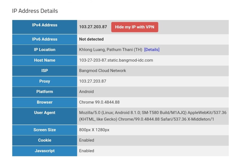
When we place the 3 devices gabriel-SM-G991B, gabriel-SM-N960F, and gabriel-SM-T580 outside the home network, either in a different WiFi network or in a mobile network and connect to the Linux server via the VPN services, then, because of the routing policy defined above, the devices will appear in:
- Portugal (gabriel-SM-G991B)
- Singapore (gabriel-SM-N960F)
- Thailand (gabriel-SM-T580)
We can test this with one of the websites that display IP geolocation, for example [13], and the result will look like this:
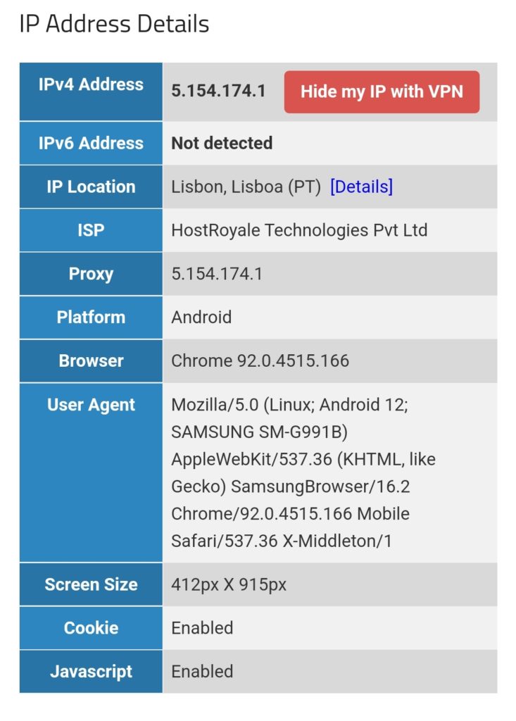
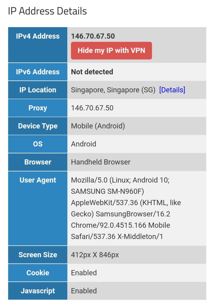
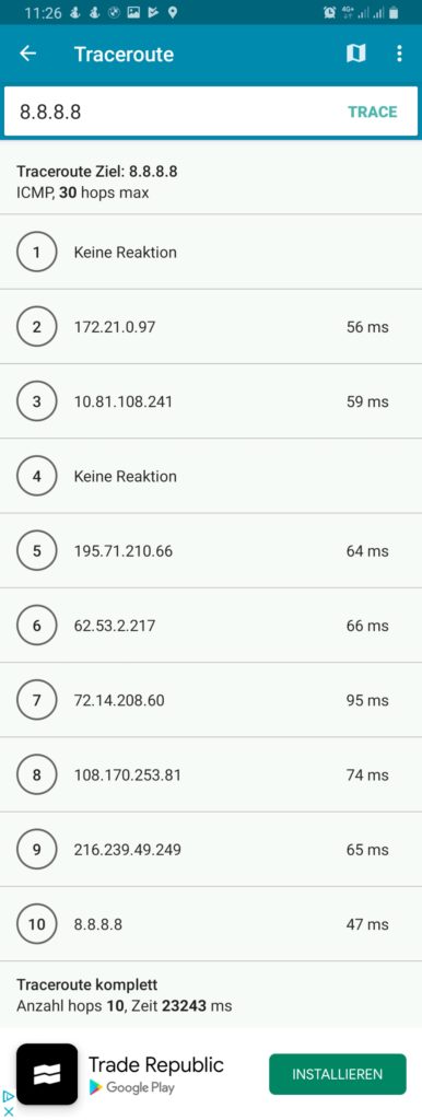
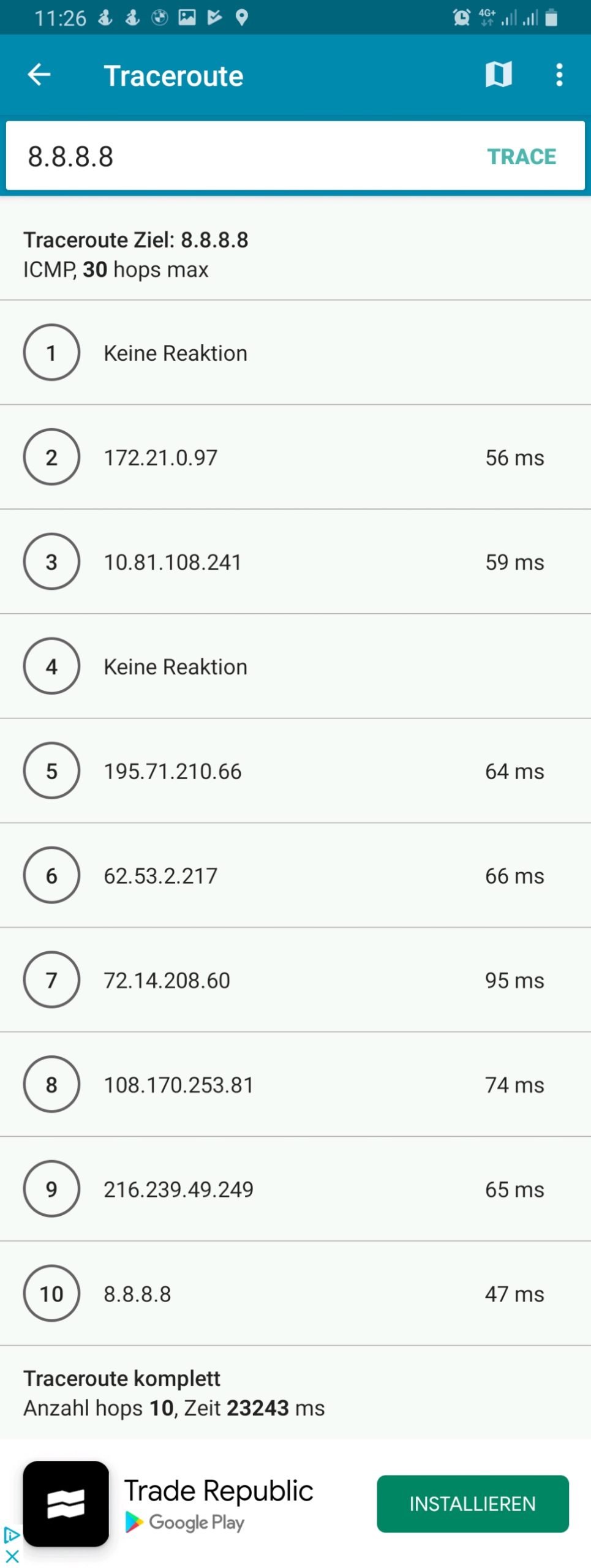
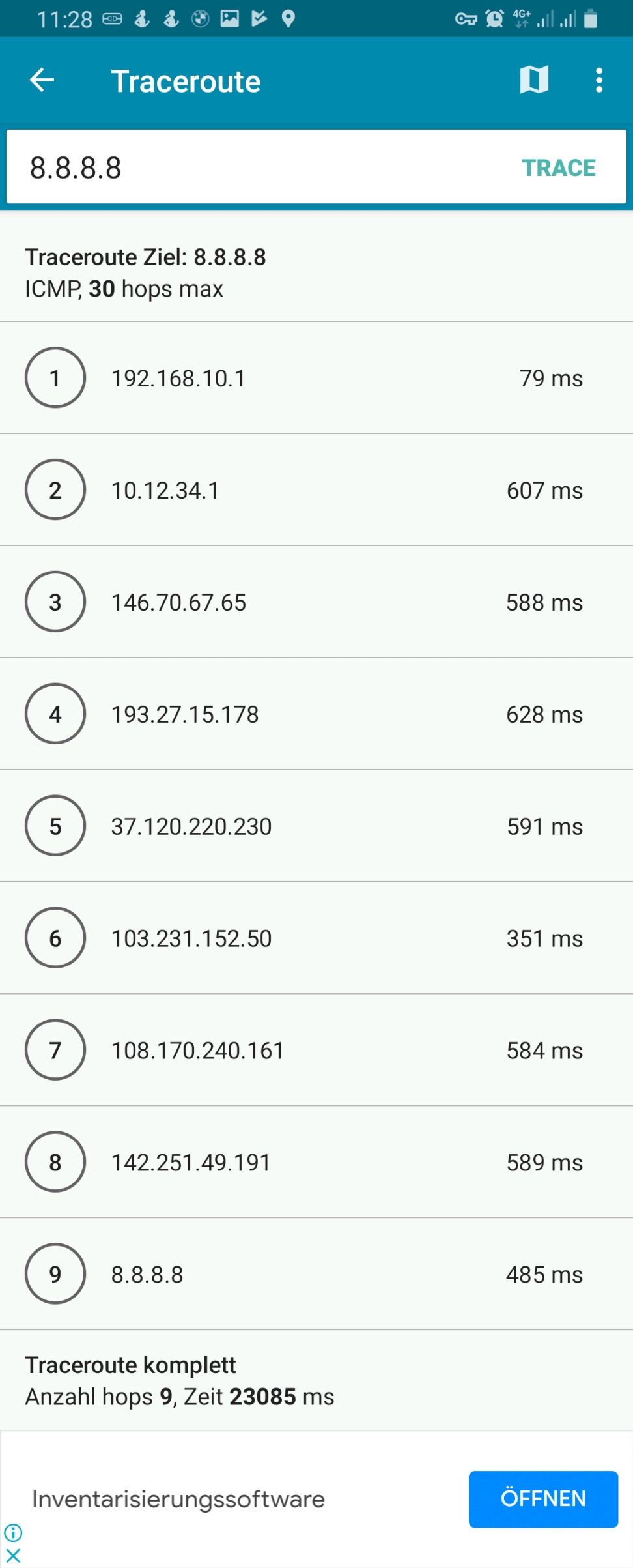
We must keep in mind that this kind of routing policy routes all outgoing traffic from the 3 devices to the respective countries, irrespective whether this is web or email or any other traffic. This is true for any protocol, and so, a traceroute to Google‘s DNS (8.8.8.8) will really go via the respective country. The images below compare the device gabriel-SM-N960F without VPN (4G mobile network) and with the VPN to the Linux server which then routes the connection via Singapore. One can easily recognize the much higher latency via Singapore. The traceroutes were taken with [14].

Policy Routing with Firewall Marking
While the ip-rule command [11] already offers a lot of possible combinations for the selection of packets, sometimes, one needs more elaborate selection criteria. This is when we use policy routing using firewall marking and the mangle table [15]. We first delete our rule set from above with the sequence:
ip rule del from 192.168.10.250/32 table Portugal priority 2000
ip rule del from 192.168.10.251/32 table Singapur priority 2000
ip rule del from 192.168.10.252/32 table Thailand priority 2000
Then, we enter new rules. Instead of using IP addresses in the selector, we use a so-called “firewall mark” (fwmark). We tell the Linux server to process packets that have a special mark in the routing tables mentioned in the action field of ip-rule:
ip rule add from all fwmark 0x1 priority 5000 lookup Portugal
ip rule add from all fwmark 0x2 priority 5000 lookup Singapur
ip rule add from all fwmark 0x3 priority 5000 lookup Thailand
But how do we mark packets? This is done in the mangle table, one of the 4 tables of the iptables [12] command. With command listed below we specify the marking of TCP packets originating from the listed IP address and going to the destination ports 80 (http) and 443 (https). All other traffic from the device with the listed IP address (e.g., smtp, imap, UDP, ICMP, …) will not be marked.
iptables -t mangle -F
iptables -t mangle -A PREROUTING -j CONNMARK --restore-mark
iptables -t mangle -A PREROUTING -m mark ! --mark 0 -j ACCEPT
iptables -t mangle -A PREROUTING -s 192.168.10.250/32 -p tcp -m multiport --dports 80,443 -m state --state NEW,RELATED -j MARK --set-mark 1
iptables -t mangle -A PREROUTING -s 192.168.10.251/32 -p tcp -m multiport --dports 80,443 -m state --state NEW,RELATED -j MARK --set-mark 2
iptables -t mangle -A PREROUTING -s 192.168.10.252/32 -p tcp -m multiport --dports 80,443 -m state --state NEW,RELATED -j MARK --set-mark 3
iptables -t mangle -A PREROUTING -j CONNMARK --save-mark
Let us have a closer look at the 7 iptables commands:
- This command flushes all chains of the mangle table so that the mangle table is empty.
- This command restores the marks of packets. Here, one must know that the mark of a packet is not stored in the packet itself, as the IP header does not contain a field for such a mark. Rather than that, the Linux Kernel keeps track of the mark and the packet it belongs to. However, when the Linux server sends out a packet to its destination, and the computer at the destination (e.g., a web server) answers with his own packets, then when these packets arrive at our Linux server, we want to mark them, too, because they belong to a data connection whose packets were initially marked and we might need the mark in order to process them correctly. Therefore, we “restore” the mark in the PREROUTING chain of the mangle table.
- This command accepts all packets that have a non-zero mark. I am not really sure if that command is needed at all (should be tested).
- This command sets the mark “1” to those packets that fulfil all these requirements:
- It comes from the source IP address 192.168.10.250.
- It uses TCP.
- It goes to one of the destination ports 80 (http) or 443 (https).
- It constitutes a NEW or RELATED connection.
- This command sets the mark “2” to those packets that fulfil all these requirements:
- It comes from the source IP address 192.168.10.251.
- It uses TCP.
- It goes to one of the destination ports 80 (http) or 443 (https).
- It constitutes a NEW or RELATED connection.
- This command sets the mark “3” to those packets that fulfil all these requirements:
- It comes from the source IP address 192.168.10.252.
- It uses TCP.
- It goes to one of the destination ports 80 (http) or 443 (https).
- It constitutes a NEW or RELATED connection.
- This command stores in the mark of the packets in the connection tracking table.
After we have entered these commands, the mangle table should look somewhat like this:
caipirinha:/etc/openvpn # iptables -t mangle -L -n -v
Chain PREROUTING (policy ACCEPT 210K packets, 106M bytes)
 pkts bytes target     prot opt in     out     source               destination
 953K  384M CONNMARK   all  --  *      *       0.0.0.0/0            0.0.0.0/0            CONNMARK restore
 177K   88M ACCEPT     all  --  *      *       0.0.0.0/0            0.0.0.0/0            mark match ! 0x0
  989 76505 MARK       tcp  --  *      *       192.168.10.250       0.0.0.0/0            multiport dports 80,443 state NEW,RELATED MARK set 0x1
 1233 82791 MARK       tcp  --  *      *       192.168.10.251       0.0.0.0/0            multiport dports 80,443 state NEW,RELATED MARK set 0x2
 1017 72624 MARK       tcp  --  *      *       192.168.10.252       0.0.0.0/0            multiport dports 80,443 state NEW,RELATED MARK set 0x3
 776K  296M CONNMARK   all  --  *      *       0.0.0.0/0            0.0.0.0/0            CONNMARK save

Chain INPUT (policy ACCEPT 203K packets, 104M bytes)
 pkts bytes target     prot opt in     out     source               destination

Chain FORWARD (policy ACCEPT 137K packets, 69M bytes)
 pkts bytes target     prot opt in     out     source               destination

Chain OUTPUT (policy ACCEPT 199K packets, 107M bytes)
 pkts bytes target     prot opt in     out     source               destination

Chain POSTROUTING (policy ACCEPT 335K packets, 176M bytes)
 pkts bytes target     prot opt in     out     source               destination
The values in the columns pkts, bytes will most probably be different in your case. They show how many IP packets and bytes have matched this rule and can help in controlling or debugging the configuration and the traffic flows.
The entries in the mangle table consequently mark the packets that traverse our Linux router and that are from one of the devices gabriel-SM-G991B, gabriel-SM-N960F, or gabriel-SM-T580 and that are destined to a web server (TCP ports 80, 443) with either the fwmark “1”, “2”, or “3”. Based on this fwmark, the packets are then sent to the routing tables Portugal, Singapur or Thailand. Using both the routing policy database and the mangle table is a powerful instrument for selecting packets and connections that shall be routed in a special way which gives us a lot of flexibility.
For example, if we only had one device to be considered (Gabriel-SM-G991B), the two command that we have issues before:
ip rule add from all fwmark 0x1 priority 5000 lookup Portugal
iptables -t mangle -A PREROUTING -s 192.168.10.250/32 -p tcp -m multiport --dports 80,443 -m state --state NEW,RELATED -j MARK --set-mark 1
have the same effect as these two commands:
ip rule add from 192.168.10.250/32 fwmark 0x1 priority 5000 lookup Portugal
iptables -t mangle -A PREROUTING -p tcp -m multiport --dports 80,443 -m state --state NEW,RELATED -j MARK --set-mark 1
In the first case, the source address selection is done in the iptables command, in the second case it is done in the ip rule command. With the 3 devices that have, the second way is not a solution as it would create the fwmark “1” on all packets that go to a web server and the subsequent entries in the mangle table would not be executed any more. We therefore have to create rules with extreme caution, in order not to jeopardize our intended routing behavior. I therefore recommend being as specific as possible already in the iptables command, also in order to avoid excessive packet marking as this complicates your life when you have to debug your setup.
When we have the setup described in this chapter active, the 3 devices (gabriel-SM-G991B, gabriel-SM-N960F, gabriel-SM-T580) will appear to be in the respective countries, similar to the setup in the previous chapter where we only modified the routing policy database. We can test this with one of the websites that display IP geolocation, for example [13], and the result will look like this:
However, if we execute a traceroute command on one of the devices, the traceroute does not go via the respective country because it uses the protocol ICMP rather than TCP and is therefore not marked and consequently is not routed via any of the client VPNs. This can be seen in the rightest image in the following gallery where a traceroute to Google‘s DNS (8.8.8.8) has been made. The traceroutes were taken with [14].

Connection Tracking
In the previous chapter, the iptables statements for the mangle table apply to NEW or RELATED connections only. Let us therefore look into the concept of connection tracking [4], [21]. This is achieved by the netfilter component [16] which is linked to the Linux Kernel keeps track of stateful connections in the connection tracking table, very similar to a stateful firewall [17]. Important states are [4]:
- NEW: The packet does not belong to an existing connection.
- ESTABLISHED: The packet belongs to an “established” connection. A connection is changed from NEW to ESTABLISHED when it receives a valid response in the opposite direction.
- RELATED: Packets that are not part of an existing connection but are associated with a connection already in the system are labeled RELATED. An example are ftp connections which open connections adjacent to the initial one [18].
- INVALID: Packets can be marked INVALID if they are not associated with an existing connection and are not appropriate for opening a new connection.
The mighty conntrack toolset [19] contains the command conntrack [20] which can be used to see the connection tracking table (actually, there are also different tables) and to inspect various behaviors around the connection tracking table. We can, for example, examine which connections have the fwmark “2” set, that is, which connections have been set up by the device Gabriel-Tablet using the source IP address 192.168.10.251:
caipirinha:/etc/openvpn # conntrack -L -m2
tcp      6 431952 ESTABLISHED src=192.168.10.251 dst=172.217.19.74 sport=38330 dport=443 src=172.217.19.74 dst=10.12.42.37 sport=443 dport=38330 [ASSURED] mark=2 use=1
tcp      6 431832 ESTABLISHED src=192.168.10.251 dst=34.107.165.5 sport=38924 dport=443 src=34.107.165.5 dst=10.12.42.37 sport=443 dport=38924 [ASSURED] mark=2 use=1
tcp      6 431955 ESTABLISHED src=192.168.10.251 dst=142.250.186.170 sport=58652 dport=443 src=142.250.186.170 dst=10.12.42.37 sport=443 dport=58652 [ASSURED] mark=2 use=1
tcp      6 65 TIME_WAIT src=192.168.10.251 dst=142.250.185.66 sport=57856 dport=443 src=142.250.185.66 dst=10.12.42.37 sport=443 dport=57856 [ASSURED] mark=2 use=1
tcp      6 431954 ESTABLISHED src=192.168.10.251 dst=142.250.186.170 sport=58640 dport=443 src=142.250.186.170 dst=10.12.42.37 sport=443 dport=58640 [ASSURED] mark=2 use=1
conntrack v1.4.5 (conntrack-tools): 5 flow entries have been shown.
Each line contains a whole set of information which is explained in detail in [2], § 7. For a quick orientation, we have to know the following points:
- Each line has two parts. The first part lists the IP header information of the newly initiated connection; in our case, we observe:
- The source IP address is always 192.168.10.251 (Gabriel-Tablet).
- The destination port is either 80 or 443 as we change the routing for exactly these destination ports only
- The second part lists the IP header information of the expected or received (as an answer) packets, and, we observe:
- The source IP address of the answering packet is the destination IP address of the initiating packet which makes sense.
- The source port of the answering packet is the destination port of the initiating packet which again makes sense.
- The destination IP address of the answering packet is not 192.168.10.251, but 10.12.42.37. This is because 10.12.42.37 is the IP address of the tun1 device of the Linux server. When we send out the initiating packet from 192.168.10.251, the packet will go to the Linux server who acts as router. In the server, the packet will be changed, and the server will use its source address on the outgoing interface tun1 as source address on the packet as the remote end point of the client VPN connection that we use would not know how to route a packet to 192.168.10.251 (the remote end point does not know anything of the network 192.168.10.0/24 on our side).
- [ASSURED] means that the connection has already seen traffic in both directions, the connections has therefore been set up successfully.
- Coincidentally, in our example, we only have TCP connections; however, the connection tracking table can also comprise UDP or ICMP connections.
The command conntrack [20] offers much more opportunities and even allows to change entries in the connection tracking table. So, we barely scratched the surface.
Conclusion
In this blog post, we have used client VPN connections to execute some experiments on policy routing in which we make different devices appear to be located in different countries. We touched the concepts of routing tables, the routing policy database, the mangle table, and the connection tracking table. The possibilities of all these items go far beyond of what we discussed in this blog post. The interested reader is referred to the sources listed below to get in-depth knowledge and to understand the vast possibilities that these items offer to the expert.
Sources
- [1] = Linux Advanced Routing & Traffic Control HOWTO
- [2] = Iptables Tutorial 1.2.2
- [3] = Guide to IP Layer Network Administration with Linux
- [4] = A Deep Dive into Iptables and Netfilter Architecture
- [5] = Policy Routing With Linux – Online Edition
- [6] = Understanding modern Linux routing (and wg-quick)
- [7] = Netfilter Connmark
- [8] = Internet Censorship in China
- [9] = Reference manual for OpenVPN 2.4
- [10] = man 8 wg-quick
- [11] = man 8 ip-rule
- [12] = man 8 iptables
- [13] = Where is my IP location? (Geolocation)
- [14] = PingTools Network Utilities [Google Play]
- [15] = Mangle table for iptables
- [16] = The netfilter.org project
- [17] = Stateful firewall [Wikipedia]
- [18] = Active FTP vs. Passive FTP, a Definitive Explanation
- [19] = The conntrack-tools user manual
- [20] = man 8 conntrack
- [21] = Connection tracking
Setting up Dual Stack VPNs
Executive Summary
This blog post explains how I set up dual stack (IPv4, IPv6) virtual private networks (VPN) with the open-source packages openvpn and WireGuard on my Linux server caipirinha.spdns.org. Clients (smartphones, tablets, notebooks) which connect to my server will be supplied with a dual stack VPN connection and can therefore use both IPv4 as well as IPv6 via the Linux server to the internet.
Background
The implementation was originally intended to help a friend who lived in China and who struggled with his commercial VPN that only tunneled IPv4 and did not block IPv6. He often experienced blockages when he tried to access social media sites as his system would prefer IPv6 over IPv4 and so the connection would not run through his VPN. However, due to [6], openvpn alone is no longer suited to circumvent censorship in China [7]. WireGuard might still work in geographies where openvpn is blocked, however.
Preconditions
In order to use the approach described here, you should:
- … have a full dual stack internet connection (IPv4, IPv6)
- … have access to a Linux machine which is already properly configured for dual stack on its principal network interface (e.g., eth0)
- … have the Linux machine set up as a router
- … have the package openvpn and/or WireGuard installed (preferably from a repository of your Linux distribution)
- … know how to create client and server certificates for openvpn [11] and/or WireGuard [12], [13], [19] although this blog post will also contain a short description on how to create a set of certificates and keys for openvpn
- … have knowledge of routing concepts, networks, some understanding of shell scripts and configuration files
- … know related system commands like sysctl
Description and Usage
The graph below shows the setup on my machine caipirinha.spdns.org with 5 VPN services (blue, green color) that will be described in this blog post. The machine has also 3 VPN clients configured which are mapped to a commercial service (ocker color), but this will not be topic of this blog post.
Home Network Setup
Let us now look at some details of the network setup:
- The Linux server is not connected to the internet directly, but it is connected to a small SoHo router which acts as basic firewall and forwards a selection of ports and protocols to the Linux server.
- The internal IPv4 network which is setup by the SoHo router is 192.168.2.0/24.
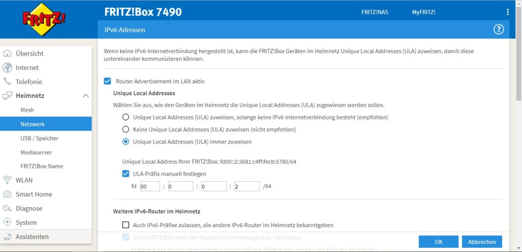
- The internal IPv6 network which is setup by the SoHo router is fd00:0:0:2/64; this is configured in the respective menu of the SoHo router as shown below and is within the IPv6 unique local address space [1], [2]. I decided to use an IPv6 with a “2” in the network address like the “2” in the IPv4 network.
- The Linux server also gets a public IPv6 address allocated (like all other devices in my home network); this is accomplished by the SoHo router that has IPv6 enabled.
When everything has been set up correctly, the Linux server should get various IP addresses, and among them various IPv6 addresses:
- a “real” and routable one starting with numbers in the range from “2000:” until “3fff:”.
- a SLAAC [3] one starting with “fe80:”
- a “private” one starting with “fd00::2:”
An example is shown here:
caipirinha:~ # ifconfig eth0
eth0: flags=4163 mtu 1500
inet 192.168.2.3 netmask 255.255.255.0 broadcast 192.168.2.255
inet6 2001:16b8:306c:c700:76d4:35ff:fe5c:d2c3 prefixlen 64 scopeid 0x0
inet6 fe80::76d4:35ff:fe5c:d2c3 prefixlen 64 scopeid 0x20
inet6 fd00::2:76d4:35ff:fe5c:d2c3 prefixlen 64 scopeid 0x0
...
Enabling Routing
Routing for IPv4 and IPv6 needs to be enabled on the Linux server. I personally also decided to switch off the privacy extensions on the Linux server, but that is a personal matter of taste:
# Enable "loose" reverse path filtering and prohibit icmp redirects
sysctl -w net.ipv4.conf.all.rp_filter=2
sysctl -w net.ipv4.conf.all.send_redirects=0
sysctl -w net.ipv4.conf.eth0.send_redirects=0
sysctl -w net.ipv4.icmp_errors_use_inbound_ifaddr=1

# Enable IPv6 routing, but keep SLAAC for eth0
sysctl -w net.ipv6.conf.eth0.accept_ra=2
sysctl -w net.ipv6.conf.all.forwarding=1

# Switch off the privacy extensions
sysctl -w net.ipv6.conf.eth0.use_tempaddr=0
OpenVPN Key Management with Easy-RSA
For the openVPN server and clients, we need a certification authority and we ultimately need to create signed certificates and keys. This can be done with the help of the package easy-rsa that is available for various platforms [22] and often is part of Linux distributions, too. Documentation and hands-on examples are given in [20] and [21].
We start with the initialization of a Public Key Infrastructure (PKI) and the creation of a Certificate Authority (CA) followed by the creation of a Certificate Revocation List (CRL)
easyrsa init-pki
easyrsa build-ca nopass
easyrsa gen-crl
The next step is the creation of a key pair for the server. The public key will be signed by the CA and thus become our server certificate. Furthermore, we create Diffie-Hellman parameters for the server (not needed if you create elliptic keys). All this can be done by:
easyrsa --days=3652 build-server-full caipirinha.spdns.org nopass
easyrsa gen-dh
In this example, the server certificate is valid for some 3652 days (10 years), the certificate is named caipirinha.spdns.org.crt, and the private key which must remain on the server is named caipirinha.spdns.org.key.
Now, we can create client certificates in a similar way. In the example, the client certificates will have a validity of 5 years only:
easyrsa --days=1825 build-client-full gabriel-SM-G991B nopass
easyrsa --days=1825 build-client-full gabriel-SM-N960F nopass
easyrsa --days=1825 build-client-full gabriel-SM-N915FY nopass
easyrsa --days=1825 build-client-full gabriel-SM-T580 nopass
...
I chose not to use passwords for the private key in order to facilitate the handling. Furthermore, I went for the easy way and created all certificates and keys on one system only. If you intend to deploy a professional solution, you have to keep cyber-security in mind and you may therefore want to exercise more caution and separate the certificate authority on a secured system from the creation of server and client key pairs as it has been advised in [20].
OpenVPN Server Configuration
Before we go into details of the configuration, we must distinguish 3 concepts of VPNs:
- A (full) tunneling VPN tunnels all connections through the VPN, once the VPN connection has been established. This offers possibilities, but also has implications:
- The VPN client appears to be in the geographic location of the VPN server unless the server itself tunnels through more nodes. This can be useful to circumvent censorship in the geography where the VPN client is located as all connections from the client to services in the internet are channeled through the VPN server.
- In a complex multi-level server setup, it can make the client appear in different countries, depending on which destination the client is trying to access. A VPN client might, for example, be in Angola, but connect to a VPN server in Germany which itself has VPN connections to Brazil and to Portugal. If the VPN server is configured accordingly, the VPN client in Angola may appear as being in Portugal when accessing Portuguese web sites and might appear as being located in Brazil when accessing Brazilian web sites and might appear as being located in Germany for everything else.
- The VPN server can implement filtering services like filtering out ad servers or doing virus scans of downloads.
- The VPN server can implement access restrictions; companies use this sometimes to disallow clients to access web sites which they deem to be related to “sex, hate, crime, gambling, …”.
- A split tunneling VPN tunnels only connections to certain networks between the VPN client and the VPN server while all other connections from the VPN client access the internet through the local provider. The typical usage scenario is not related to censorship, but to dedicated resources to which the VPN server grants access (e.g., network shares aka “samba”, proxy services, etc.) that shall be accessed from the VPN client while the latter is not physically connected to the home or company network.
- An inverse split tunneling VPN tunnels almost all connections, with a few exceptions. This concept is often used in companies which want basically all connections to run through their infrastructure so that they can execute virus scans and access restrictions, but which have (correctly) realized that bandwidth-intensive operations like cloud access, access to video conferencing services, etc. should be taken off the VPN tunnel as their performance is deteriorated otherwise.
The following configurations will create 4 different VPNs based on 2 concepts above.
- UDP-based VPN, full tunneling: This is the preferred VPN when all connections shall be tunneled.
- UDP-based VPN, split tunneling: This is the preferred VPN when you want to blend in resources from your home network.
- TCP-based VPN, full tunneling: TCP can be used when the connection quality to the VPN server is unstable or when UDP is blocked by some gateway in between.
- TCP-based VPN, split tunneling: This is the preferred VPN when you want to blend in resources from your home network, but when the connection quality to the VPN server is unstable or when UDP is blocked by some gateway in between.
UDP-based VPN, full tunneling
# Konfigurationsdatei für den openVPN-Server auf CAIPIRINHA (UDP:1194)

ca                    /root/pki/ca.crt
cert                  /etc/openvpn/caipirinha.spdns.org.crt
client-config-dir     /etc/openvpn/conf-1194
crl-verify            /root/pki/crl.pem
dev                   tun4
dh                    /root/pki/dh.pem
hand-window           90
ifconfig              192.168.10.1  255.255.255.0
ifconfig-pool         192.168.10.2  192.168.10.239  255.255.255.0
ifconfig-ipv6         fd01:0:0:a::1 fd00::2:3681:c4ff:fecb:5780
ifconfig-ipv6-pool    fd01:0:0:a::2/112
ifconfig-pool-persist /etc/openvpn/ip-pool-1194.txt
keepalive             20 80
key                   /etc/openvpn/caipirinha.spdns.org.key
log                   /var/log/openvpn-1194.log
mode                  server
persist-key
persist-tun
port                  1194
proto                 udp6
reneg-sec             86400
script-security       2
status                /var/run/openvpn/status-1194
tls-server
topology              subnet
up                    /etc/openvpn/start_vpn.sh
verb                  1
writepid              /var/run/openvpn/server-1194.pid

# Topologie des VPN und Default-Gateway
push "topology subnet"
push "route-gateway 192.168.10.1"
push "redirect-gateway def1 bypass-dhcp"
push "tun-ipv6"
push "route-ipv6 2000::/3"
# DNS-Server
push "dhcp-option DNS 8.8.8.8"
push "dhcp-option DNS 8.8.4.4"
UDP-based VPN, split tunneling
# Konfigurationsdatei für den openVPN-Server auf CAIPIRINHA (UDP:4396)

ca                    /root/pki/ca.crt
cert                  /etc/openvpn/caipirinha.spdns.org.crt
client-config-dir     /etc/openvpn/conf-4396
crl-verify            /root/pki/crl.pem
dev                   tun7
dh                    /root/pki/dh.pem
hand-window           90
ifconfig              192.168.13.1  255.255.255.0
ifconfig-pool         192.168.13.2  192.168.13.239  255.255.255.0
ifconfig-ipv6         fd01:0:0:d::1 fd00::2:3681:c4ff:fecb:5780
ifconfig-ipv6-pool    fd01:0:0:d::2/112
ifconfig-pool-persist /etc/openvpn/ip-pool-4396.txt
keepalive             20 80
key                   /etc/openvpn/caipirinha.spdns.org.key
log                   /var/log/openvpn-4396.log
mode                  server
persist-key
persist-tun
port                  4396
proto                 udp6
reneg-sec             86400
script-security       2
status                /var/run/openvpn/status-4396
tls-server
topology              subnet
up                    /etc/openvpn/start_vpn.sh
verb                  1
writepid              /var/run/openvpn/server-4396.pid

# Topologie des VPN und Default-Gateway
push "topology subnet"
push "route-gateway 192.168.13.1"
push "tun-ipv6"
push "route-ipv6 2000::/3"
# Routen zum internen Netzwerk setzen
push "route 192.168.2.0 255.255.255.0"
TCP-based VPN, full tunneling
# Konfigurationsdatei für den openVPN-Server auf CAIPIRINHA  (TCP:8080)

ca                    /root/pki/ca.crt
cert                  /etc/openvpn/caipirinha.spdns.org.crt
client-config-dir     /etc/openvpn/conf-8080
crl-verify            /root/pki/crl.pem
dev                   tun5
dh                    /root/pki/dh.pem
hand-window           90
ifconfig              192.168.11.1  255.255.255.0
ifconfig-pool         192.168.11.2  192.168.11.239  255.255.255.0
ifconfig-ipv6         fd01:0:0:b::1 fd00::2:3681:c4ff:fecb:5780
ifconfig-ipv6-pool    fd01:0:0:b::2/112
ifconfig-pool-persist /etc/openvpn/ip-pool-8080.txt
keepalive             20 80
key                   /etc/openvpn/caipirinha.spdns.org.key
log                   /var/log/openvpn-8080.log
mode                  server
persist-key
persist-tun
port                  8080
proto                 tcp6-server
reneg-sec             86400
script-security       2
status                /var/run/openvpn/status-8080
tls-server
topology              subnet
up                    /etc/openvpn/start_vpn.sh
verb                  1
writepid              /var/run/openvpn/server-8080.pid

# Topologie des VPN und Default-Gateway
push "topology subnet"
push "route-gateway 192.168.11.1"
push "redirect-gateway def1 bypass-dhcp"
push "tun-ipv6"
push "route-ipv6 2000::/3"
# DNS-Server
push "dhcp-option DNS 8.8.8.8"
push "dhcp-option DNS 8.8.4.4"
TCP-based VPN, split tunneling
# Konfigurationsdatei für den openVPN-Server auf CAIPIRINHA  (TCP:8081)

ca                    /root/pki/ca.crt
cert                  /etc/openvpn/caipirinha.spdns.org.crt
client-config-dir     /etc/openvpn/conf-8081
crl-verify            /root/pki/crl.pem
dev                   tun6
dh                    /root/pki/dh.pem
hand-window           90
ifconfig              192.168.12.1  255.255.255.0
ifconfig-pool         192.168.12.2  192.168.12.239  255.255.255.0
ifconfig-ipv6         fd01:0:0:c::1 fd00::2:3681:c4ff:fecb:5780
ifconfig-ipv6-pool    fd01:0:0:c::2/112
ifconfig-pool-persist /etc/openvpn/ip-pool-8081.txt
keepalive             20 80
key                   /etc/openvpn/caipirinha.spdns.org.key
log                   /var/log/openvpn-8081.log
mode                  server
persist-key
persist-tun
port                  8081
proto                 tcp6-server
reneg-sec             86400
script-security       2
status                /var/run/openvpn/status-8081
tls-server
topology              subnet
up                    /etc/openvpn/start_vpn.sh
verb                  1
writepid              /var/run/openvpn/server-8081.pid

# Topologie des VPN und Default-Gateway
push "topology subnet"
push "route-gateway 192.168.12.1"
push "tun-ipv6"
push "route-ipv6 fd00:0:0:2::/64"
# Routen zum internen Netzwerk setzen
push "route 192.168.2.0 255.255.255.0"
We shall now look at some configuration parameters and their meaning:
- cert, key: The location of the server certificate and the server key has to be listed.
- ca: The location of the certificate authority certificate has to be listed.
- crl-verify: This point to a certificate revocation list and contains the certificates that once were issued for devices that have been retired meanwhile or for users that only needed a temporary VPN access .
- dev: This determines the tun device that shall be used for the connection. I recommend using dedicated tun devices for all VPNs rather than having them randomly assigned during start-up.
- ifconfig, ifconfig-pool: This determines the IPv4 address of the server and the pool from which IPv4 addresses are granted to the clients. I decided to use a different /24 network for each VPN configuration, that is, the networks 192.168.10.0/24, 192.168.11.0/24, 192.168.12.0/24, and 192.168.13.0/24. However, I decided not to use the full IP address range for dynamic allocation as I have some VPN clients (smartphones, notebooks) which get a dedicated client address so that I can easily tweak settings on the Linux server for those clients. These clients have a small, dedicated configuration file in the folder named in client-config-dir. Such a dedicated configuration can be used to allocate the same IP address to a certain VPN client.
- ifconfig-ipv6: The first parameter is the IPv6 address of the server, and the second IPv6 address is the one of the router to the internet; in that case, I put the SoHo router there (fd00::2:3681:c4ff:fecb:5780), see the image Configuration of the internal IPv6 network.
- ifconfig-ipv6-pool: This is the pool of IPv6 addresses that are granted to the clients. I follow a similar approach as with the IPv4 networks and set up separate networks for each VPN, that is, the networks fd01:0:0:a::2/112, fd01:0:0:b::2/112, fd01:0:0:c::2/112 and fd01:0:0:d::2/112. Keep in mind that the first address of the IP address pool is the one mentioned here, e.g., fd01:0:0:a:0:0:0:2, as fd01:0:0:a:0:0:0:1 is already used for the server.
- keepalive: Sets the interval of ping-alive requests and its timeout. This is useful as gateways that are in between the VPN client and the VPN server might keep connections open and port allocations reserved only for some time; subsequently, they might be freed up. Ideally, you want to use the longest time periods possible as shorter periods create unnecessary traffic (and might eat up the data volume of mobile clients).
- port: While the standard port for openvpn is 1194, with more than one VPN you are better advised to use different, dedicated ports that are not used by other service on your server.
- proto: This determines the protocol used and is either udp6 or tcp6-server. The “6” in both arguments indicates that the service shall be provided both on the IPv4 as well as on the IPv6 address. Leaving the “6” away only provides the service on the IPv4 address.
- push “redirect-gateway def1 bypass-dhcp” tells the VPN client to bypass the VPN for DHCP queries. Otherwise, the client machine gets stuck when the DHCP lease on the client side terminates.
- push “route-ipv6 2000::/3” tells the VPN client machine to use the VPN for all IPv6 addresses that start with “2000::/3”, and those are currently all routable IPv6 addresses [2].
- push “dhcp-option DNS 8.8.8.8” and push “dhcp-option DNS 8.8.4.4” set Google‘s DNS servers for the VPN client machine and so gives us an excellent and fast service.
- reneg-sec: The specified 86400 seconds re-negotiate new encryption keys only once per day. For security reasons, a lower time period would be better, but some countries have put in efforts to detect and block encrypted communication, and this detection happens though the key exchange which seems to have a characteristic bit pattern [6]; therefore, a longer period has been set here.
OpenVPN Client Configuration
The generation of client configuration files is explained in [11], and there are numerous guidelines in the internet. Therefore, I just want to give 2 examples and briefly point out some useful considerations.
UDP-based VPN, full tunneling
# Konfigurationsdatei für den openVPN-Client auf ...

client
dev              tun
explicit-exit-notify
hand-window      90
keepalive        10 60
nobind
persist-key
persist-tun
proto            udp
remote           caipirinha.spdns.org 1194
remote-cert-tls  server
reneg-sec        86400
script-security  2
verb             1

<ca>
-----BEGIN CERTIFICATE-----
MIIE2D...NNmlTg=
-----END CERTIFICATE-----
</ca>

<cert>
-----BEGIN CERTIFICATE-----
MIIFJj...nbuzbI=
-----END CERTIFICATE-----
</cert>

<key>
-----BEGIN PRIVATE KEY-----
MIIEvA...QcO+Q==
-----END PRIVATE KEY-----
</key>
TCP-based VPN, full tunneling
# Konfigurationsdatei für den openVPN-Client auf ...

client
dev              tun
hand-window      90
keepalive        10 60
nobind
persist-key
persist-tun
proto            tcp
remote           caipirinha.spdns.org 8080
remote-cert-tls  server
reneg-sec        86400
script-security  2
verb             1

<ca>
-----BEGIN CERTIFICATE-----
MIIE2D...NNmlTg=
-----END CERTIFICATE-----
</ca>

<cert>
-----BEGIN CERTIFICATE-----
MIIFJj...nbuzbI=
-----END CERTIFICATE-----
</cert>

<key>
-----BEGIN PRIVATE KEY-----
MIIEvA...QcO+Q==
-----END PRIVATE KEY-----
</key>
The following points proved to be useful for me:
- Rather than using separate files for the ca, the certificate, and the key of the client, all information can actually be packed into one file which then gives a complete configuration of the client. This eases the installation on mobile clients (smartphones, tablets) as you do not have to consider path names on the target device. For security reasons, the respective code blocks are not printed here.
- It is possible to use several remote statements. You can refer to different servers (if the client configuration is suitable for the servers) or you can name the very same server with different ports. On my server, I have different ports open which all point to the very same 4 different server processes. The reason is that sometimes, the dedicated openvpn port 1194 is blocked in some geographies, but other ports might still work. In that case, you have to ensure that connections coming to all these ports are mapped back to the port of the server process. And you might include the statement remote-random so that one connection of the ones listed is chosen randomly.
- On the client, is it normally not necessary to bind the openvpn process to a certain tun device or a certain port, different from the VPN server.
Further Improvements (OpenVPN)
Different network conditions might require tweaking one or the other parameters of the openvpn service. [8], [9], [10] contain some indications, especially with respect to different hardware and network conditions.
Dedicated Configurations
As mentioned above, the client-config-dir directive can be used to refer to a folder that contains configurations for dedicated devices. An example is the file /etc/openvpn/conf-1194/Gabriel-SM960F. It contains the content:
# Spezielle Konfigurationsdatei für Gabriels Galaxy Note 9 (gabriel-SM-N960F)
#

ifconfig-push      192.168.10.251  255.255.255.0
ifconfig-ipv6-push fd01:0:0:a:0:0:1:fb/111 fd01:0:0:a::1
This file makse the device with the client certificate named gabriel-SM-N960F always receive the same IP addresses, namely 192.168.10.251 (IPv4) and fd01:0:0:a:0:0:1:fb (IPv6). The name of the file must exactly match the VPN client’s common name (CN) that was defined when the client certificate was created [5].
WireGuard Server Configuration
WireGuard is a new and promising VPN protocol [15] which is not yet as widespread as openvpn; it may therefore “escape” censorship authorities easier than openvpn which can be detected by statistical analysis [16]. The setup of the server is described in [12], [13], a more complex configuration is described in [19]. A big advantage of WireGuard is also that the code base is very lean, and hence performance on any given platform is higher than with openvpn.
I personally find it unusual that you have to list the clients in the server configuration file rather than just having a general server configuration where any number of allowed clients can connect to. On my Linux server caipirinha.spdns.org, the WireGuard server configuration contains of 3 files:
- /etc/wireguard/wg_caipirinha_public.key is the public key of the service (the generation is described in [12], [13], [19]).
- /etc/wireguard/wg_caipirinha_private.key is the private key of the service (the generation is described in [12], [13], [19]).
- /etc/wireguard/wg0.conf is the configuration file (the network device is named “wg0” on my machine).
Similar to the openvpn configurations described above, I spent a dedicated IPv4 and IPv6 subnet for the WireGuard server, in this case 192.168.14.0/24 and fd01:0:0:e::/64. The configuration file /etc/wireguard/wg0.conf is easy to understand and contains important parameters that shall be discussed below:
[Interface]
Address = 192.168.14.1/24,fd01:0:0:e::1/64
ListenPort = 44576
PrivateKey = SHo...

[Peer]
PublicKey = pjp2PEboXA4RJhVoybXKuicNkz4XDZaW+c9yLtJq1gE=
AllowedIPs = 192.168.14.2/32,fd01:0:0:e::2/128
PersistentKeepalive = 30
...
[Peer]
PublicKey = fcEcFYQ6cOqe7H9L2PvkM78mkKottJLnKwiqp4WO91s=
AllowedIPs = 192.168.14.7/32,fd01:0:0:e::7/128
PersistentKeepalive = 30
...
The section [Interface] describes the server setup:
- Address lists the server’s IPv4 and IPv6 addresses.
- ListenPort is the UDP port on which the service will listen.
- PrivateKey is the private server key (can be read from the file /etc/wireguard/wg_caipirinha_private.key). For security reasons, the key has only been displayed partly here.
Each section [Peer] lists a possible client configuration. If you want to enable 10 clients on your server, you therefore need 10 such sections.
- PublicKey is the public key of the client.
- AllowedIPs lists the IPv4 and IPv6 addresses which will be allocated to the client upon connection.
- PersistentKeepalive configures the time in seconds after which “keep-alive packets” will be exchanged between the server and the client. This helps to keep connection settings on gateways that are in between the VPN client and the VPN server open; often firewalls and routers in between might otherwise delete the connection from their tables. A value of 25…30 is recommended.
WireGuard Client Configuration
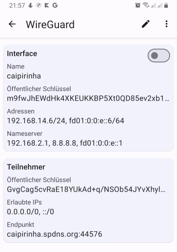
WireGuard clients exist for all major operating systems. I would like to show a Windows 10 configuration that I set up on one of my notebooks according to [14].

As we can see, I also named the respective network interface on the client wg0, but you can use any other name, too. The detailed configuration of the only client connection is also easy to understand:
[Interface]
PrivateKey = 2B2...
Address = 192.168.14.7/32, fd01:0:0:e::7/128
DNS = 192.168.14.1, fd01:0:0:e::1

[Peer]
PublicKey = GvgCag5cvRaE18YUkAd+q/NSOb54JYvXhylm1oz8OxI=
AllowedIPs = 0.0.0.0/0, ::/0
Endpoint = caipirinha.spdns.org:44576
The section [Interface] describes the client setup:
- PrivateKey is the private key of the client which is generated in the application itself [14]. For security reasons, the key has only been displayed partly here.
- Address lists the client’s IPv4 and IPv6 addresses.
- DNS lists the DNS servers which shall be used when the VPN connection is active. In this case, the Linux server caipirinha.spdns.org has a DNS service running, hence I listed the server IPv4 and IPv6 addresses here. You might also use Google’s DNS with the IPv4 addresses 8.8.8.8, 8.8.4.4, for example. It is important to list the DNS servers as the ones that you were using before the VPN was established (e.g., the router’s IP like 192.168.4.1) might no longer be accessible after the VPN has been established.
The section [Peer] contains information related to the server.
- PublicKey is the public key of the server which is located on the server in the file /etc/wireguard/wg_caipirinha_public.key.
- AllowedIPs is set to 0.0.0.0/0, ::/0 on this client which means that all traffic shall be sent via the VPN (fully tunneling VPN). Here, you have the chance to move from a fully tunneling VPN to a split VPN by listing subnets like 192.168.2.0/24, for example.
- Endpoint lists the server FQDN and the port to which the client shall connect to.
In a similar way, I set up another client on an Android smartphone using the official WireGuard – Apps bei Google Play, following the configuration model at [23].
Let’s see how that works out in reality. For the experiment, I am in Brazil and connect to my Linux server caipirinha.spdns.org in Germany with the configurations described above. Once, the connection has been established, I do a traceroute in Windows to www.google.com in IPv4 and IPv6:
C:\Users\Dell>tracert www.google.com

Routenverfolgung zu www.google.com [142.250.185.68]
über maximal 30 Hops:

  1   235 ms   236 ms   236 ms  CAIPIRINHA [192.168.14.1]
  2   241 ms   238 ms   238 ms  Router-EZ [192.168.2.1]
  3   259 ms   248 ms   249 ms  fra1813aihr002.versatel.de [62.214.63.145]
  4   250 ms   249 ms   248 ms  62.214.38.105
  5   249 ms   247 ms   249 ms  72.14.204.149
  6   249 ms   250 ms   251 ms  72.14.204.148
  7   249 ms   249 ms   248 ms  108.170.236.175
  8   251 ms   249 ms   250 ms  142.250.62.151
  9   248 ms   247 ms   247 ms  fra16s48-in-f4.1e100.net [142.250.185.68]

Ablaufverfolgung beendet.

C:\Users\Dell>tracert -6 www.google.com

Routenverfolgung zu www.google.com [2a00:1450:4001:829::2004]
über maximal 30 Hops:

  1   235 ms   235 ms   235 ms  fd01:0:0:e::1
  2   239 ms   239 ms   237 ms  2001:16b8:30b3:f100:3681:c4ff:fecb:5780
  3   249 ms   249 ms   247 ms  2001:1438::62:214:63:145
  4   248 ms   249 ms   247 ms  2001:1438:0:1::4:302
  5   250 ms   248 ms   248 ms  2001:1438:1:1001::1
  6   250 ms   249 ms   248 ms  2001:1438:1:1001::2
  7   252 ms   250 ms   249 ms  2a00:1450:8163::1
  8   250 ms   249 ms   250 ms  2001:4860:0:1::5894
  9   248 ms   250 ms   251 ms  2001:4860:0:1::5009
 10   250 ms   249 ms   249 ms  fra24s06-in-x04.1e100.net [2a00:1450:4001:829::2004]

Ablaufverfolgung beendet.

C:\Users\Dell>
We can see a couple of interesting points:
- The latency from Brazil to my server is already > 200 ms, that is not a very competitive connection.
- Despite the fact that between my Linux server caipirinha.spdns.org and Google, there are a range of machines, that connections has quite a low (additional) latency.
Let’s now switch off the VPN and do a traceroute to www.google.com directly from the local ISP:
C:\Users\Dell>tracert www.google.com

Routenverfolgung zu www.google.com [172.217.29.100]
über maximal 30 Hops:

  1    <1 ms    <1 ms    <1 ms  fritz.box [192.168.4.1]
  2     1 ms    <1 ms    <1 ms  192.168.100.1
  3     4 ms     4 ms     3 ms  179-199-160-1.user.veloxzone.com.br [179.199.160.1]
  4     5 ms     5 ms     4 ms  100.122.52.96
  5    12 ms     6 ms     5 ms  100.122.25.245
  6    11 ms    11 ms    11 ms  100.122.17.180
  7    12 ms    12 ms    12 ms  100.122.18.52
  8    12 ms    11 ms    11 ms  72.14.218.158
  9    14 ms    13 ms    14 ms  108.170.248.225
 10    15 ms    14 ms    14 ms  142.250.238.235
 11    13 ms    13 ms    13 ms  gru09s19-in-f100.1e100.net [172.217.29.100]

Ablaufverfolgung beendet.
For this test, only IPv4 was possible as I did not have IPv6 connection at the Ethernet port where my notebook was connected to. The overall connection is much faster, and we can clearly identify that it uns in the Brazilian internet (“179-199-160-1.user.veloxzone.com.br”).
Further Improvements (WireGuard)
A range of graphical user interfaces (GUIs) for the configuration of WireGuard have come up that seek to overcome the need to deal with various configuration files on the server and the client side and align public keys and IP addresses. [17] compares some GUIs for WireGuard, [18] shows a further possibility.
Configuring Network Address Translation (NAT)
Additionally, to the configuration of the VPNs (and their respective start on the VPN server), we need to set up network address translation so that connections from the VPN networks are translated to the SoHo network. This is done with the sequence:
readonly STD_IF='eth0'
…
iptables -t nat -F
iptables -t nat -A POSTROUTING -s 192.168.10.0/24 -o ${STD_IF} -j MASQUERADE
iptables -t nat -A POSTROUTING -s 192.168.11.0/24 -o ${STD_IF} -j MASQUERADE
iptables -t nat -A POSTROUTING -s 192.168.12.0/24 -o ${STD_IF} -j MASQUERADE
iptables -t nat -A POSTROUTING -s 192.168.13.0/24 -o ${STD_IF} -j MASQUERADE
iptables -t nat -A POSTROUTING -s 192.168.14.0/24 -o ${STD_IF} -j MASQUERADE
…

# Setup the NAT table for the VPNs.
ip6tables -t nat -F
ip6tables -t nat -A POSTROUTING -s fd01:0:0:a::/64 -o ${STD_IF} -j MASQUERADE
ip6tables -t nat -A POSTROUTING -s fd01:0:0:b::/64 -o ${STD_IF} -j MASQUERADE
ip6tables -t nat -A POSTROUTING -s fd01:0:0:c::/64 -o ${STD_IF} -j MASQUERADE
ip6tables -t nat -A POSTROUTING -s fd01:0:0:d::/64 -o ${STD_IF} -j MASQUERADE
ip6tables -t nat -A POSTROUTING -s fd01:0:0:e::/64 -o ${STD_IF} -j MASQUERADE
...
Conclusion
The VPN configuration mentioned above shows how to set up different VPNs that allow dual stack operations on a Linux server. Thus, VPN clients can initiate connections in IPv4 or IPv6 mode using the assigned IP addresses from a private address space; the configured network address translation (NAT) translates the connections to a real-world IP address on the server.
Outlook
The VPN server itself can also act as VPN client itself, and so, the connection from the original VPN client can be forwarded via other VPNs to other countries allowing the original VPN client to appear in different geographies depending upon the destination address of its outgoing connection. This can be useful in order to circumvent geo-blocking of media content, for example.
Sources
- [1] = Unique local address [Wikipedia]
- [2] = IPv6: Basics
- [3] = Stateless address autoconfiguration (SLAAC)
[4] = OpenVPN / easy-rsa-old [Github](superseded)- [5] = Instalando e configurando o OpenVPN
- [6] = OpenVPN Traffic Identification Using Traffic Fingerprints and Statistical Characteristics
- [7] = Internet Censorship in China
- [8] = Improving OpenVPN performance and throughput
- [9] = Optimizing OpenVPN Throughput
- [10] = Optimizing performance on gigabit networks
- [11] = Setting up your own Certificate Authority (CA) and generating certificates and keys for an OpenVPN server and multiple clients
- [12] = WireGuard Quick Start
- [13] = How to setup a VPN server using WireGuard (with NAT and IPv6)
- [14] = How to configure a WireGuard Windows 10 VPN client
- [15] = WireGuard vs OpenVPN: 7 Big Difference
- [16] = OpenVPN Traffic Identification Using Traffic Fingerprints and Statistical Characteristics
- [17] = Wireguard GUIs im Vergleich
- [18] = WireGuard VPN Server mit Web Interface einrichten
- [19] = WireGuard [ArchWiki]
- [20] = Home – Easy RSA (easy-rsa.readthedocs.io)
- [21] = Easy-RSA – ArchWiki (archlinux.org)
- [22] = GitHub – OpenVPN/easy-rsa: easy-rsa – Simple shell based CA utility
- [23] = DualStack VPN mit Wireguard – sebastian heg.ge
Colored Network Diagrams (Part 2)
Executive Summary
This blog post is the continuation of the blog post Colored Network Diagrams (Part 1). In this blog post, I describe some improvements and enhanced capabilities of the scripts that have been presented in Part 1 already. The new set of scripts can now additionally color network graphs (PERT charts) according to:
- … remaining durations
- … remaining work
- … criticality based on remaining duration
Before reading this blog post, you need to read the blog post Colored Network Diagrams (Part 1) first to fully understand the context.
Preconditions
In order to use the approach described here, you should:
- … have access to a Linux machine or account
- … have a MySQL or MariaDB database server set up, running, and have access to it
- … have the package graphviz [2] installed
- … have some basic knowledge of how to operate in a Linux environment and some basic understanding of shell scripts
Description and Usage
In the previous blog post Colored Network Diagrams (Part 1) we looked at a method on how to create colored network graphs (PERT charts) based on the duration, the work, the slack, and the criticality of the individual tasks. We also looked at how a network graph looks like when some of the tasks have already been completed (tasks in green color). We will now enhance the script sets in order to process remaining duration and remaining work. In addition, this information shall also be displayed for each task. For this, the scripts create_project_db.sql, msp2mysql.sh, and mysql2dot.sh require modifications so that they can process the additional information. I decided to name the new scripts with a “-v2” suffix so that they can be distinguished from the ones in the previous blog post.
Let us first look at the script create_project_db-v2.sql which sets up the database [1]. Compared to the previous version, it now sets up some new fields which have been highlighted in red color below. For the sake of readability, only parts of the script have been displayed here.
...
task_duration INT UNSIGNED DEFAULT 0,\
task_work INT UNSIGNED DEFAULT 0,\
free_slack INT DEFAULT 0,\
total_slack INT DEFAULT 0,\
finish_slack INT DEFAULT 0,\
rem_duration INT UNSIGNED DEFAULT 0,\
rem_work INT UNSIGNED DEFAULT 0,\
`%_complete`
In addition to the fields rem_duration and rem_work, we also prepare the database for 3 out of the 4 slack types that tasks have (free_slack, total_slack, finish_slack), in order to be able to execute some experiments in future releases. Furthermore, we can now capture the link_lag between two linked tasks; this information will not be used now, but in a future version of the script set.
Step 1: Parsing the Project Plan
The script msp2mysql-v2.sh parses the Microsoft® Project plan in XML format. It contains a finite-state machine (see graph below), and the transitions between the states are XML tags (opening ones and closing ones).
Step 2: Generating a Graph
Now we can extract meaningful data from the database and transform this into a colored network graph; this is done with the bash script mysql2dot-v2.sh. mysql2dot-v2.sh can create colored network graphs according to:
- … the task duration
- … the work allocated to a task
- … the total slack of a task
- … the criticality of a task
- … the remaining task duration
- … the remaining work allocated to a task
- … the remaining criticality of a task
mysql2dot-v2.sh relies on a working installation of the graphviz package, and in fact, it is graphviz and its collection of tools that create the graph, while mysql2dot-v2.sh creates a script for graphviz in the dot language. Let us look close to some examples:
Example 8: A real-world example
Example 8 was already mentioned in the blog post Colored Network Diagrams (Part 1). It is a fictious simplified project plan with development, verification, and validation activities where some tasks have already been completed. The green vertical line in the plan shows the status date.

Tasks that have been completed 100% are colored in green color across all network graphs indicating that these tasks do not require any more attention in the remaining project. While the network graphs had already been shown in the blog post Colored Network Diagrams (Part 1), they shall nevertheless ben shown again as the new script mysql2dot-v2.sh shows additional information (remaining duration, remaining work) for each task. For completed tasks, those values as well as total task slack are 0, of course.
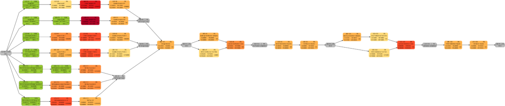
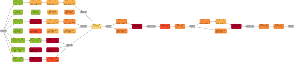
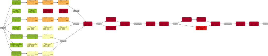

The new script mysql2dot-v2.sh offers 3 additional graphs (menu choices 5…7):
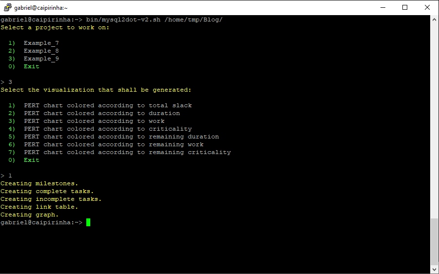
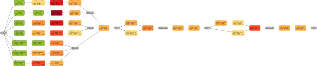
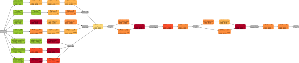
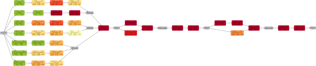
Let us have a closer look at these graphs and compare some of them:
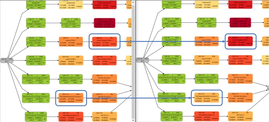
The comparison of the graphs above show two tasks whose colors have changed in different directions of color shades:
- The task with UID=116 changes to a lighter color shade. This is because the left graph takes the duration into account (D=72000), and the right graph takes the remaining duration into account (rD=36000). As the remaining duration is less than the duration, we can expect that change in the color shade.
- The task with UID=92 changes to a darker color shade although the values for the duration (D=14400) and the remaining duration (rD=14400) are equal. Why is that?
The explanation is that the spread between the color shades (the variable ${color_step} in the script mysql2dot-v2.sh) is computed based on the maximum remaining duration in the graph on the right side, different from the maximum duration in the graph on the left side. Consequently, if there is a task with a very long duration in the left graph and this task has a significantly lower remaining duration, this might occur in a smaller spread (a smaller value of ${color_step}) when the network graph for the remaining duration is computed.
I am personally open to the discussion of whether a different spread as seen in example (2) makes sense or not. For the moment, I decided to proceed like that. But there are valid arguments for both approaches:
- Leaving the spread equal between both graphs makes them directly comparable 1:1. This might be important for users who regularly compare the network graph colored according to task duration with the one colored according to remaining task duration.
- Computing the spread from scratch for each graph sets a clear focus on the tasks which should be observed now because they have a long remaining duration, irrespective of whether the tasks once in the past had a longer or shorter duration.
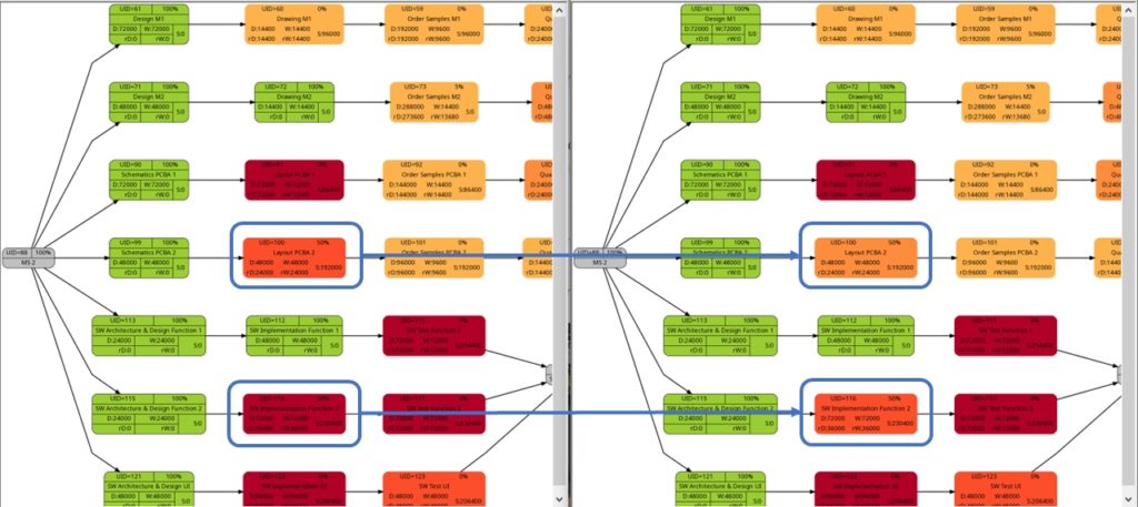
The shift of color shades in the graph above seems logical and corresponds to the case (1) of the previous example. For both the tasks with UID=100 and UID=116, the value of the remaining task work is half the value of the task work, and therefore, in the network graph for the remaining task work, both tasks feature lighter color shades as they are “less problematic”.
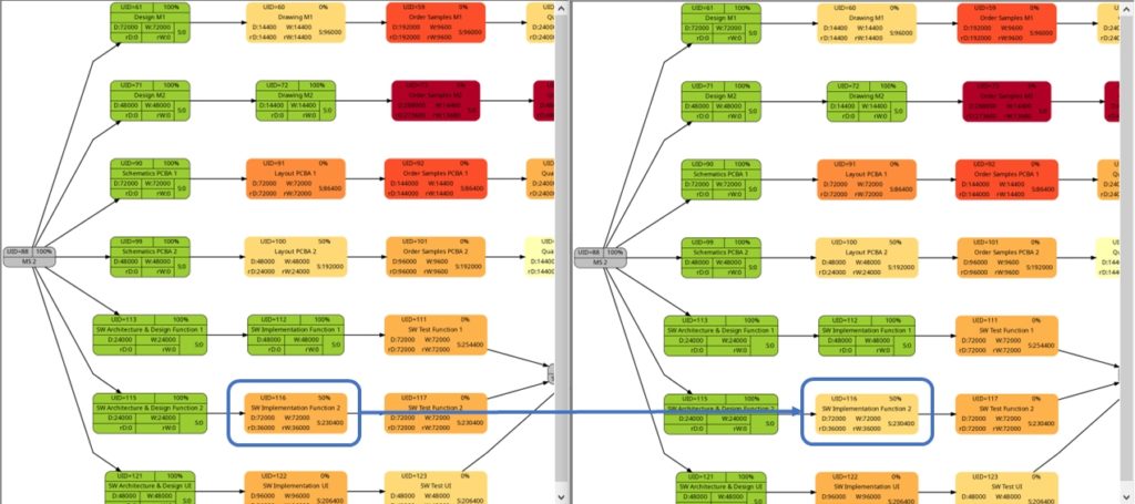
As already explained in the blog post Colored Network Diagrams (Part 1), criticality is computed based on the information of task slack and task duration. Whereas the script mysql2dot.sh used the task finish slack for this calculations, I decided to change to task total slack in the newer script mysql2dot-v2.sh; that seemed to be more adequate although in my examples, both values have been the same for all involved tasks.
In both versions of the scripts, logarithmic calculations are undertaken, and their outcome is different from the calculations based on the square root for the network graphs according to (remaining) task durations. As a result, we only observe a color shift in the task with UID=116. As the remaining task duration is half of the task duration, this task is less critical (hence, a lighter color shade) on the right side of the image above.
Example 9: Same project plan (more in the future)
Jumping to the future, more tasks of the same project plan have been completed either entirely or partially. Again, the green vertical line in the plan shows the status date.
The resulting graphs are:
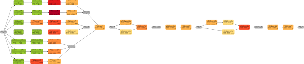
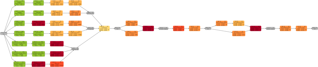
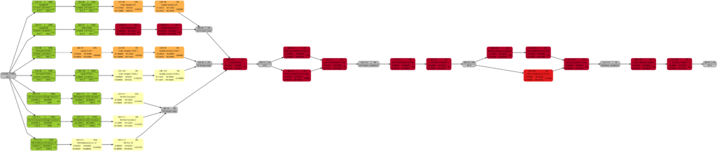
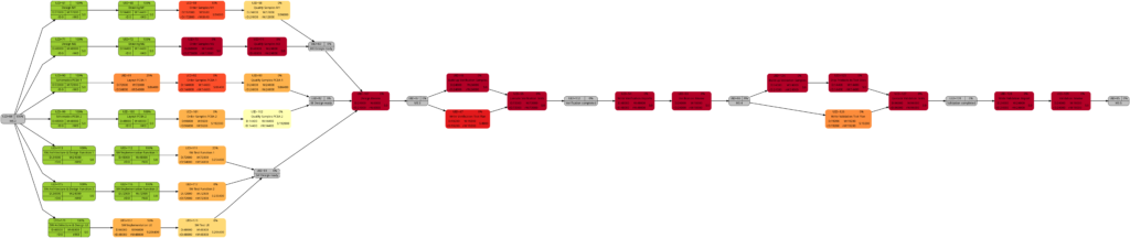
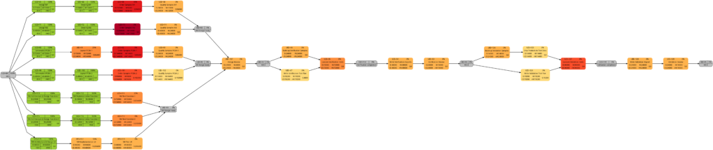
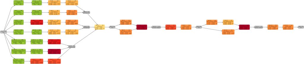
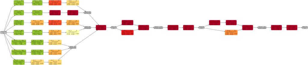
We will now look at some of the graphs and compare them with the equivalent graphs in Example 8. Apart from tasks being colored in green color once they have been completed, there are only differences in color shades of tasks belonging to the network graphs of:
- remaining task duration
- remaining task work
- remaining task criticality
as completed tasks have their remaining values set to 0 and therefore diminish the set of tasks that are considered for the calculation. In contrast to this, there are no changes in the network graphs of:
- task duration
- task work
as the respective values do not change for completed tasks. We could, however, in theory experience changes in the network graphs of:
- task slack
- task criticality
as complete tasks have their slack values set to 0 and therefore diminish the set of tasks that are considered for the calculation. This was not the case in our examples, though. It should also be mentioned that there might be changes in the color shade for a task where the duration or work is increased due to a revised assessment of the project manager from one status date to the other.
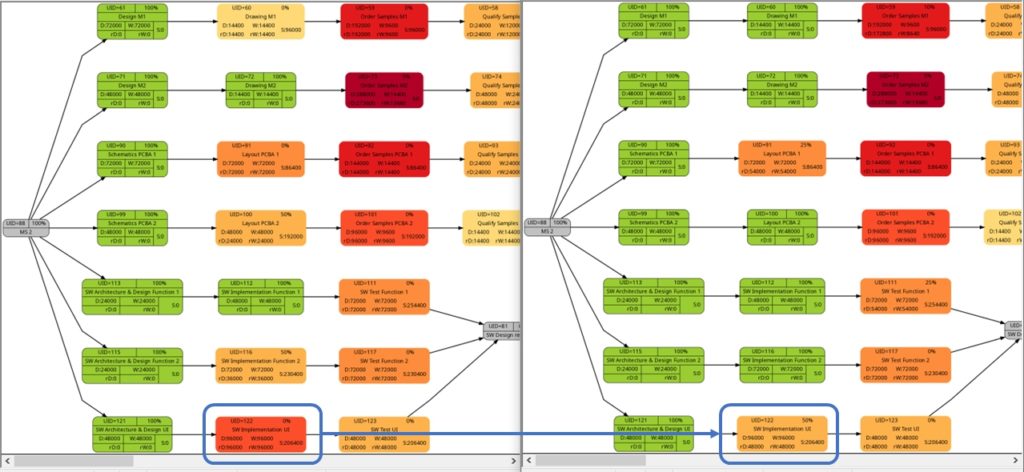
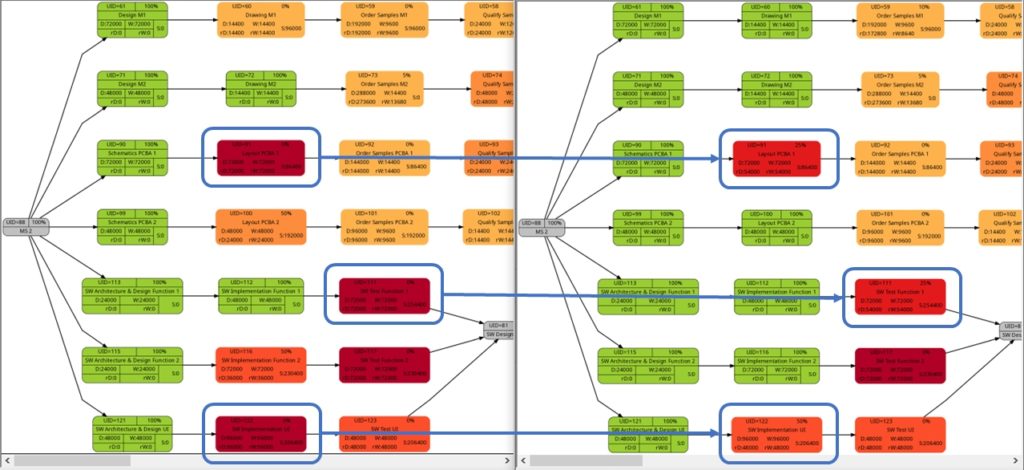
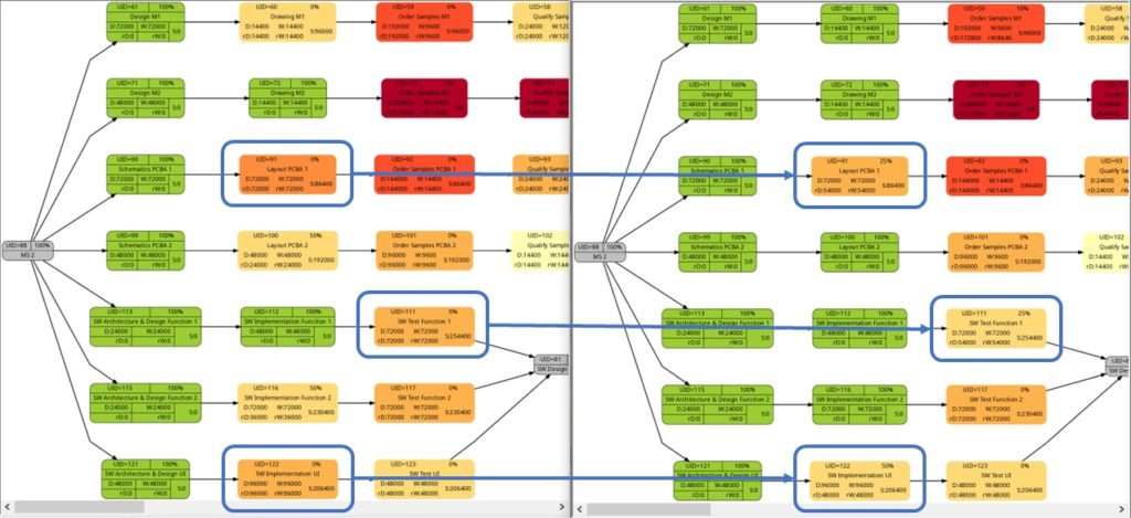
As mentioned above, the changes in the color shade of the highlighted tasks in the comparisons above are due to the fact that either the remaining duration or the remaining work of the respective tasks change between the earlier and the later status date.
Conclusion
The scripts create_project_db-v2.sql, msp2mysql-v2.sh and mysql2dot-v2.sh and the examples provided above show how, using the powerful graphviz package, traditional project plans created with Microsoft® Project can be visualized in a set of graphs that can help a project manager to focus on the right tasks. Compared to the set of scripts in the blog post Colored Network Diagrams (Part 1), the improved set of scripts additionally allow the examination of the task duration, task value, and task criticality based on remaining values of the tasks, and so can answer the question “How does the project look now?” more adequately.
Outlook
In the near future, I plan to rewrite the script mysql2dot-v2.sh into PHP because I want to incorporate an algorithm which I developed back in 2010 that can show the first x critical paths of the project using a recursive PHP function and several large multi-dimensional arrays.
Sources
Files
- create_project_db-v2.sql sets up the database in MySQL or MariaDB. The script works with the user gabriel who assumes to have access to the database server without password; you might have to adapt the script to your environment and needs.
- msp2mysql-v2.sh reads a Microsoft® Project plan in XML, parses it and writes the data into the MariaDB database.
- mysql2dot-v2.sh reads from the MariaDB database and creates a script for dot, a tool of the graphviz suite.
- Example_8-v2.zip contains all files with respect to Example 8 (created with the current set of scripts).
- Example_9-v2.zip contains all files with respect to Example 9.
Disclaimer
- The program code and the examples are for demonstration purposes only.
- The program code shall not be used in production environments without further modifications.
- The program code has not been optimized for speed (It’s a bash script anyway, so do not expect miracles.).
- The program code has not been written with cybersecurity aspects in mind.
- While the program code has been tested, it might still contain errors.
- Only a subset of all possibilities in [1] has been used, and the code does not claim to adhere completely to [1].
Colored Network Diagrams (Part 1)
Executive Summary
This blog post offers a method to create colored network graphs (PERT charts) from project plans that are created with Microsoft® Project. Color schemes similar to the ones used in physical maps visualize those tasks which:
- … have long durations
- … have a high amount work
- … have little slack
- … have a high criticality
The blog post shall also encourage readers to think outside of the possibilities that established project management software offers and to define for yourself which tasks are critical or relevant for you and how this information shall be determined.
Preconditions
In order to use the approach described here, you should:
- … have access to a Linux machine or account
- … have a MySQL or MariaDB database server set up, running, and have access to it
- … have the package graphviz installed
- … have some basic knowledge of how to operate in a Linux environment and some basic understanding of shell scripts
Description and Usage
The base for the colored network graphs is a plan in Microsoft® Project which needs to be stored as XML file. The XML file is readable with a text editor (e.g., UltraEdit) and follows the syntax in [1]. The XML file is then parsed, the relevant information is captured and is stored in a database (Step 1). Then, selected information is retrieved from the database and written to a script in dot language which subsequently is transformed into a graph using the package graphviz (Step 2). Storing the data in a database rather than in variables allows us to use all the computational methods which the database server offers in order to select, aggregate, and combine data from the project plan. It also allows us to implement Step 2 in PHP so that graphs can be generated and displayed within a web site; this could be beneficial for a web-based project information system.
Step 0: Setting up the Database
At the beginning, a database needs to be set up in the database server. For this, you will probably need administrative access to the database server. The following SQL script sets up the database and grants access rights to the user gabriel. Of course, you need to adapt this to your needs on the system you work on.
# Delete existing databases
REVOKE ALL ON projects.* FROM 'gabriel';
DROP DATABASE projects;

# Create a new database
CREATE DATABASE projects;
GRANT ALL ON projects.* TO 'gabriel';
USE projects;

CREATE TABLE projects         (proj_uid               SMALLINT UNSIGNED NOT NULL AUTO_INCREMENT PRIMARY KEY,\
                               proj_name              VARCHAR(80)) ENGINE=MyISAM DEFAULT CHARSET=utf8;
CREATE TABLE tasks            (proj_uid               SMALLINT UNSIGNED NOT NULL,\
                               task_uid               SMALLINT UNSIGNED NOT NULL,\
                               task_name              VARCHAR(150),\
                               is_summary_task        BOOLEAN           DEFAULT FALSE NOT NULL,\
                               is_milestone           BOOLEAN           DEFAULT FALSE NOT NULL,\
                               is_critical            BOOLEAN           DEFAULT FALSE NOT NULL,\
                               task_start             DATETIME          NOT NULL,\
                               task_finish            DATETIME          NOT NULL,\
                               task_duration          INT UNSIGNED      DEFAULT 0,\
                               task_work              INT UNSIGNED      DEFAULT 0,\
                               task_slack             INT               DEFAULT 0,\
                               rem_duration           INT UNSIGNED      DEFAULT 0,\
                               rem_work               INT UNSIGNED      DEFAULT 0,\
                               `%_complete`           SMALLINT UNSIGNED DEFAULT 0,\
                                                      PRIMARY KEY (proj_uid, task_uid)) ENGINE=MyISAM DEFAULT CHARSET=utf8;
CREATE TABLE task_links       (proj_uid               SMALLINT UNSIGNED NOT NULL,\
                               predecessor            SMALLINT UNSIGNED NOT NULL,\
                               successor              SMALLINT UNSIGNED NOT NULL) ENGINE=MyISAM DEFAULT CHARSET=utf8;
CREATE TABLE resources        (proj_uid               SMALLINT UNSIGNED NOT NULL,\
                               resource_uid           SMALLINT UNSIGNED NOT NULL,\
                               calendar_uid           SMALLINT UNSIGNED NOT NULL,\
                               resource_units         DECIMAL(3,2)      DEFAULT 1.00,\
                               resource_name          VARCHAR(100),\
                                                      PRIMARY KEY (proj_uid, resource_uid)) ENGINE=MyISAM DEFAULT CHARSET=utf8;
CREATE TABLE assignments      (proj_uid               SMALLINT UNSIGNED NOT NULL,\
                               task_uid               SMALLINT UNSIGNED NOT NULL,\
                               resource_uid           SMALLINT UNSIGNED NOT NULL,\
                               assignment_uid         SMALLINT UNSIGNED NOT NULL,\
                               assignment_start       DATETIME          NOT NULL,\
                               assignment_finish      DATETIME          NOT NULL,\
                               assignment_work        INT UNSIGNED      DEFAULT 0,\
                                                      PRIMARY KEY (proj_uid, task_uid, resource_uid)) ENGINE=MyISAM DEFAULT CHARSET=utf8;
CREATE TABLE assignment_data  (proj_uid               SMALLINT UNSIGNED NOT NULL,\
                               assignment_uid         SMALLINT UNSIGNED NOT NULL,\
                               assignment_start       DATETIME          NOT NULL,\
                               assignment_finish      DATETIME          NOT NULL,\
                               assignment_work        INT UNSIGNED      DEFAULT 0) ENGINE=MyISAM DEFAULT CHARSET=utf8;
This SQL script sets up a database with several tables. The database can hold several project plans, but they all must have distinctive names. This SQL script only catches a subset of all information which is part of a Microsoft® Project plan in XML format; it does not capture calendar data, for example, nor do the data types in the SQL script necessarily match the ones from the specification in [1]. But it is good enough to start with colored network graphs.
This only needs to be executed one time. Once the database has been set up properly, we only have to execute Step 1 and Step 2.
Step 1: Parsing the Project Plan
The first real step is to parse the Microsoft® Project plan in XML format; this is done with the bash script msp2mysql.sh. This program contains a finite-state machine (see graph below), and the transitions between the states are XML tags (opening ones and closing ones). This approach helps to keep the code base small and easily maintainable. Furthermore, the code base can be enlarged if more XML tags or additional details of the project plan shall be considered.
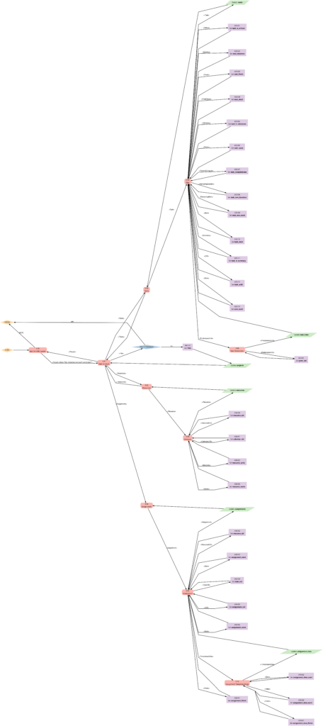
I concede there are more elegant and faster ways to parse XML data, but I believe that msp2mysql.sh can be understood well and helps to foster an understanding of what needs to be done in Step 1.
There is one important limitation in the program that needs to be mentioned: The function iso2msp () transforms a duration in ISO 8601 format to a duration described by multiples of 6 s (6 s are an old Microsoft® Project “unit” of a time duration, Microsoft® Project would traditionally only calculate with 0.1 min of resolution). However, as you can see in [2], durations cannot only be measured in seconds, minutes, and hours, but also in days, months, etc. A duration of 1 month is a different amount of days, depending on the month we are looking at. This is something that has not been considered in this program; in fact, it can only transform durations given in hours, minutes and seconds to multiples of 6 s. Fortunately, this captures most durations used by Microsoft® Project, even durations that span over multiple days (which are mostly still given in hours in the Microsoft® Project XML file).
While msp2mysql.sh parses the Microsoft® Project plan in XML format, it typically runs through these steps:
- It extracts the name of the project plan and checks if there is already a project plan with this name in the database. If that is the case, the program terminates. If that is not the case, the project name is stored in the table projects, and a new proj_uid is allocated.
- It extracts details of the tasks and stored them in the tables tasks and task_links.
- It extracts the resource names and stores their details in the table resources.
- It extracts assignments (of resources to tasks) and stores them in the tables assignments and assignment_data.
msp2mysql.sh is called with the Microsoft® Project plan in XML format as argument, like this:
./msp2mysql.sh /home/tmp/Example_1.xmlStep 2: Generating a Graph
The second step is to extract meaningful data from the database and transform this into a colored network graph; this is done with the bash script mysql2dot.sh. mysql2dot.sh can create colored network graphs according to:
- … the task duration
- … the work allocated to a task
- … the task slack
- … the criticality of a task
mysql2dot.sh relies on a working installation of the graphviz package, and in fact, it is graphviz and its collection of tools that create the graph, while mysql2dot.sh creates a script for graphviz in the dot language. Let us look close to some aspects:
mysql2dot.sh uses an uneven scale of colors, and the smallest scale should be three or more colors. The constant NUM_COLSTEPS sets the number of colors, in our case 7 colors. The constant COLSCHEME defines the graphviz color scheme that shall be used, in our case this is “ylorrd7”. [3] shows some really beautiful color schemes. The ColorBrewer schemes are well suited for our kind of purpose (or for physical maps); however, the license conditions ([4]) must be observed.
mysql2dot.sh is invoked with the name of a directory as argument. The generated script(s) in dot language as well as the generated graph(s) will be stored in that directory. A typical call looks like this:
./mysql2dot.sh /home/tmp/When started, mysql2dot.sh retrieves a list of all projects from the database and displays them to the user who then has to select a project or choose the option Exit. When a project plan has been selected, the user has to choose the graph that shall be generated. Subsequently, the program starts to generate a script in dot language and invokes the program dot (a tool of the graphviz suite) in order to compute the network graph.
Different project plans typically have different ranges of durations, work or slack for all of their tasks. mysql2dot.sh therefore takes into account the maximum duration, the maximum work, or the maximum slack it can find in the whole project. Initially, I used a linear scale to distribute the colors over the whole range from [0; max_value], but after looking at some real project plans, I personally found that too many tasks would then be colored in darker colors and I thought that this would rather distract a project manager from focusing on the few tasks that really need to be monitored closely. Trying out linear, square and square root approaches, I finally decided for the square root approach which uses the darker colors only when the slack is very small, the workload is very high, or the duration is very long. Consequently, the focus of the project manager is guided to the few tasks that really deserve special attention. However, this does not mean that this approach is the only and correct way to do it. Feel free to experience with different scaling methods to tune the outcome to your preferences.
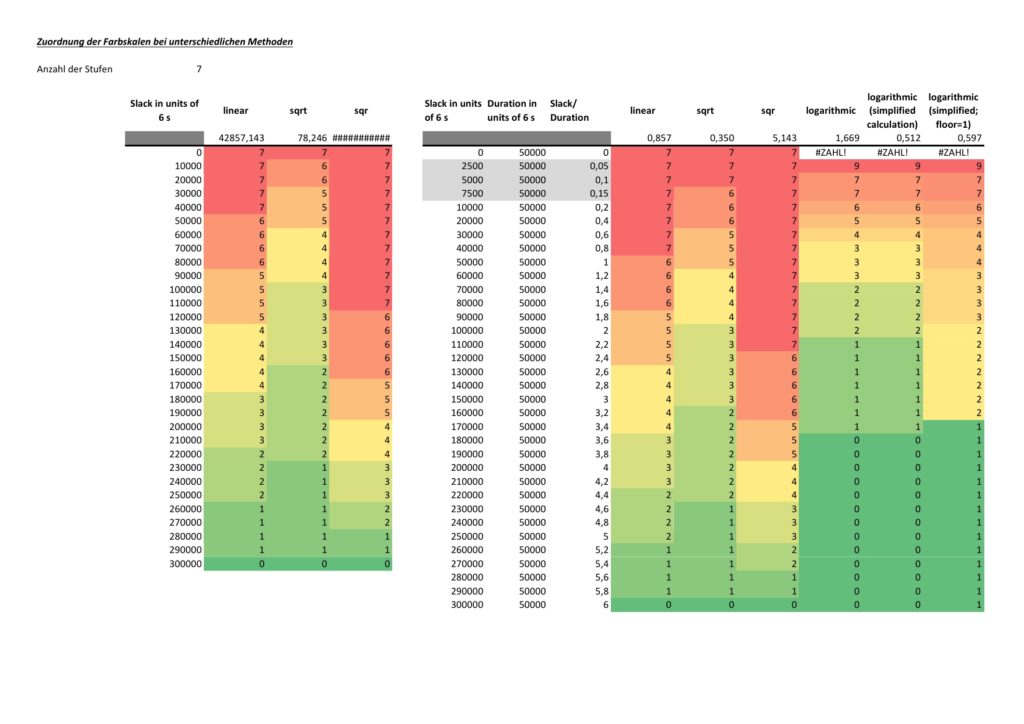
The network graph colored according to task criticality follows a different approach. Task criticality is derived from the ration of task slack and task duration. Tasks which have a low ratio of task slack / task duration are defined as more critical than tasks where this ratio is higher. I also experienced with the square root approach mentioned above, but that seemed to result in different criticalities depending on the maximum ratio of task slack / task duration which seemed unsatisfactory to me. Finally, I opted for a logarithmic approach which puts the ration task slack / task duration = 1,0 to the middle value of NUM_COLSTEPS. So in the current case, a ratio of task slack / task duration = 1,0 (means: task slack = task_duration) would result in a value of 4.0. If NUM_COLSTEPS was 9 rather than 7, the result would be 5.0. This can be reached by the formula:
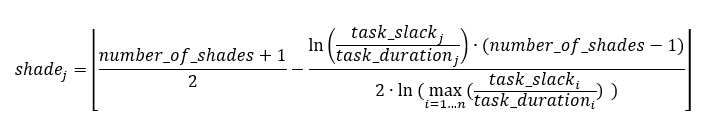
where:
- n is the number of tasks that are neither a milestone nor a summary task and that have a non-zero duration
- j is the task for which we determine the level of shade
- number_of_shades is the number of different shades you want to have in the graph; this should be an impair number and it should be 3 at least
- shadej is the numerical value of the shade for task j
- task_slackj is the task slack of task j
- task_durationj is the duration of task j
Examples
Example 1: Sequential Task Chain
This example is a sequential task chain with 20 tasks; each task is +1d longer than the previous task.
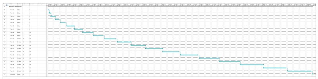
In this example, no resources have been assigned yet. As all tasks are in sequence, there is obviously no slack in any task, and all tasks are in the critical path. Parsing this project plan with msp2mysql.sh leads to:

We can already see that the shall script takes a long time for this easy project plan. For a productive environment, one would have to use C code rather than a shell script, but for educational purposes, the shell script is easier to change, understand and also to debug. Subsequently, we start creating the graphs with mysql2dot.sh, here is an example on how this looks like:
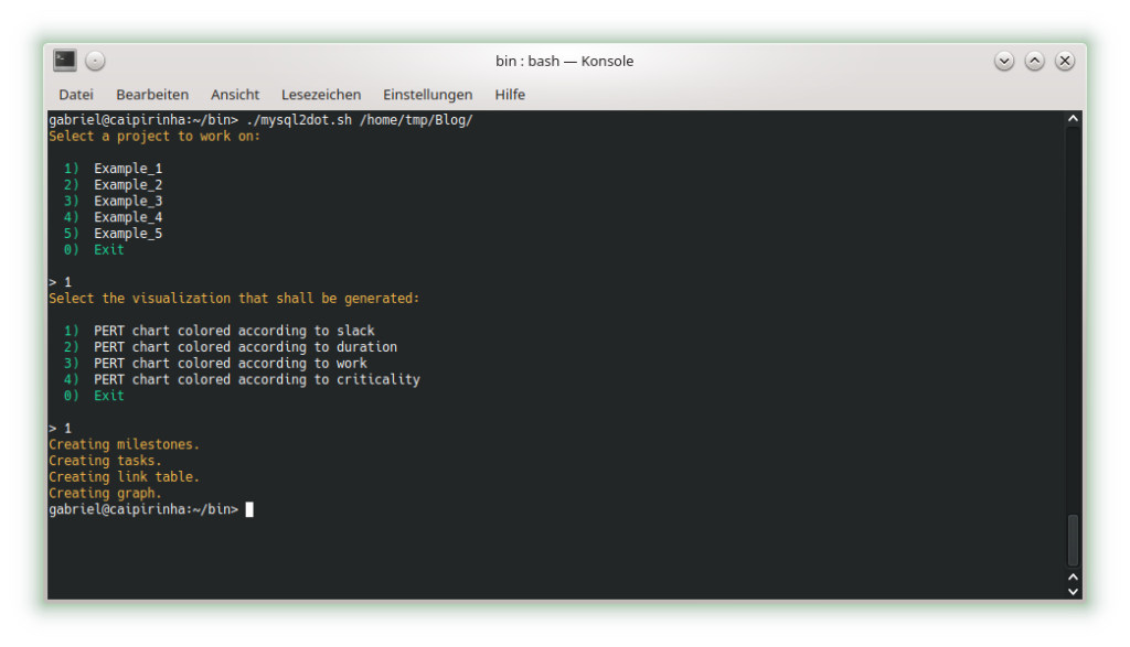
Let us look at the 4 graphs which can be generated:

The result is what could be expected. Tasks with a shorter duration are colored in a lighter color, tasks with a longer duration consequently in a darker color. While the task duration increases in a linear fashion from left to right, the graph colors tasks with a longer duration more in the “dangerous” area, that is, in a darker color.

As no resource has been attributed, no work has been registered for any of the tasks. Therefore, all tasks are equally shown in a light color.

As none of the tasks has any slack, obviously all tasks are in the critical path. Hence all of them are colored in dark color.

Similar to the graph above, all tasks are critical, and progress must be carefully monitored; hence, all tasks are colored in dark color.
Example 2: Parallel Task Chain
This example has the same tasks as Example 1, but all of them in parallel. The longest task therefore determines the overall project runtime.
In this example, too, no resources have been assigned yet. Parsing this project plan with msp2mysql.sh leads to:
The 4 graphs from this example look very different from Example 1:
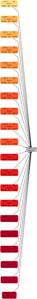
The color of the tasks is the same as in Example 1; however, all tasks are in parallel.
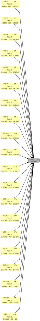
The color of the tasks is the same as in Example 1 as we still have no work assigned to any of the tasks; however, all tasks are in parallel.
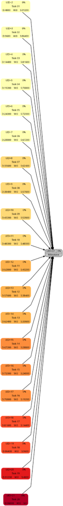
As to slack, the picture is different. Only one task (task #20) does not have any slack, all other tasks have more or less slack, and task #01 has the most slack.
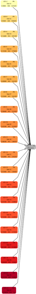
Here, we can see that both tasks #19 and tasks #20 are considered to be critical. More tasks receive a darker color as compared to the graph considering slack alone.
Example 3: Sequential Task Chain with Resource
This example has the same tasks as Example 1, but we assign a resource to each task (the same in this example, but this OK as all tasks are sequential, hence no overload of the resource). Consequently, work is assigned to each task, and we can expect changes in the network graph referring to task work.
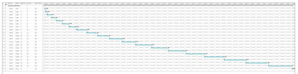
Parsing this project plan with msp2mysql.sh leads to:
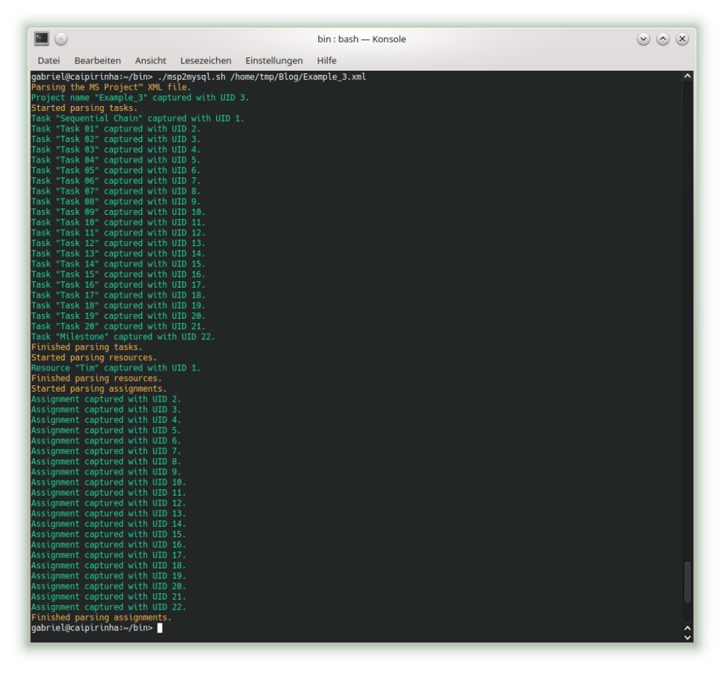
We can see that now (different from Example 1), resources and assignments are captured, too. Let us look at the 4 graphs from this example:

Nothing has changed compared to Example 1 as the durations are the same.

This graph now experiences the same coloring as the network graph according to task duration. That is understandable given the fact that we have a full-time resource working 100% of the time for the full task duration, hence work and duration have the same numeric values for each respective task.

Nothing has changed compared to Example 1 as still none of the tasks has any slack.

Nothing has changed compared to Example 1 as still none of the tasks has any slack. Consequently, all of them are critical.
Example 4: Parallel Task Chain with Resources
This example has the same tasks as Example 2, but we assign a resource to each task. As all tasks are parallel, we assign a new resource to each task so that there is no resource overload.
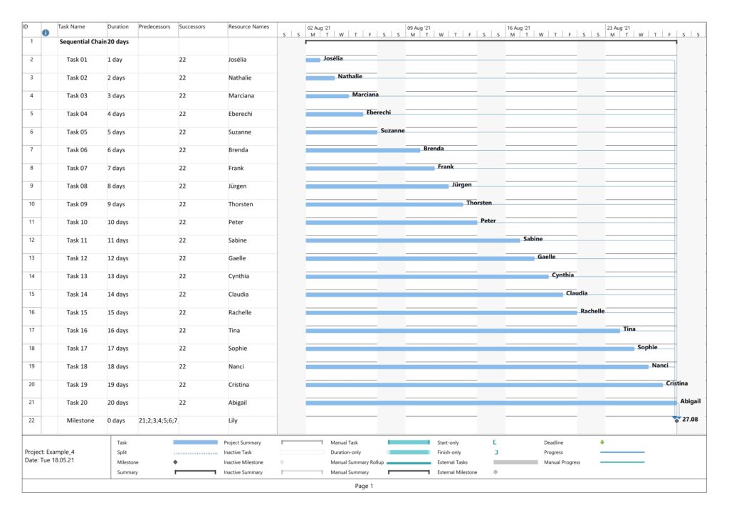
Parsing this project plan with msp2mysql.sh leads to:
We can see that now (different from Examples 2), resources and assignments are captured, too. Let us look at the 4 graphs from this example:

Nothing has changed compared to Example 2 as the durations are the same.
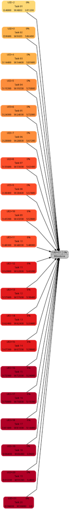
This graph now experiences the same coloring as the network graph according to task duration. That is understandable given the fact that we have a full-time resource working 100% of the time for the full task duration, hence work and duration have the same numeric values for each respective task.
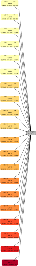
Nothing has changed compared to Example 3; the slack of each task has remained the same.
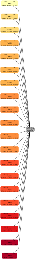
Nothing has changed compared to Example 3; the criticality of the tasks remains the same.
Example 5: Sequential Blocks with Parallel Tasks and with Resources
This example is the most interesting one as it combines different aspects within one project plan. We have 5 milestones, and 4 parallel tasks before each milestone. All tasks have resources assigned.
Task Block 1 contains 4 tasks of different durations, and as each task has a 100% resource allocated, also of different work. Due to the different durations, the 4 tasks also have different slack, with the longest task having zero slack.
Task Block 2 is like Task Block 1, but the work is the same for each task; this has been achieved by an over-allocation of the respective resources for 3 out of the 4 tasks.
Task Block 3 consists of 4 parallel tasks with the same duration, however with a work allocation similar to Task Block 1. None of the tasks therefore has slack, but the work for each task is different.
Task Block 4 is like Task Block 1 in terms of task duration and task work. However, the tasks have been arranged in a way so that none of the tasks has slack.
Task Block 5 is like Task Block 4, but each task has (the same amount of) lag time between the task end and the subsequent milestone. None of the tasks has any slack.
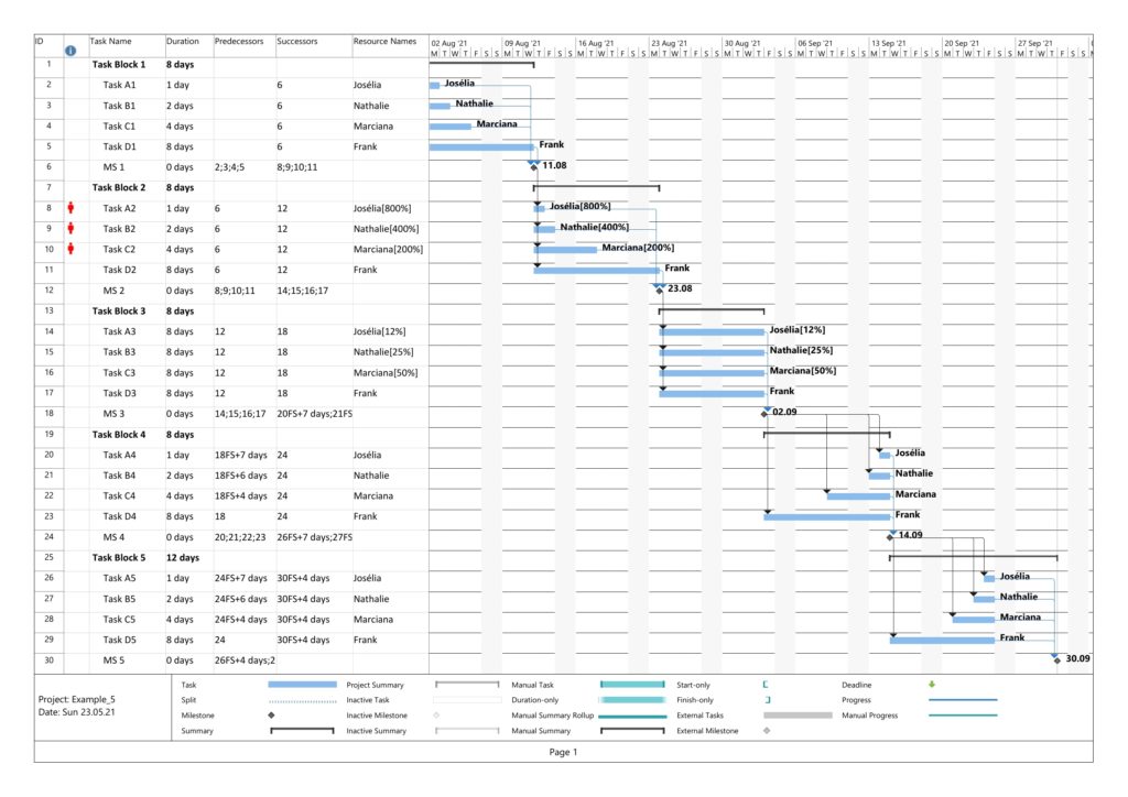
Parsing this project plan with msp2mysql.sh leads to:
Let us look at the 4 graphs from this example:
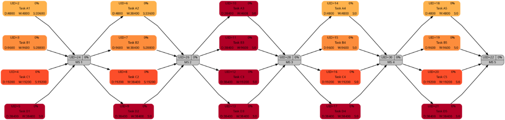
The colors in Task Block 1, 2, 4 and 5 are the same. Only in Task Block 3 where all tasks have the same (long) duration, all tasks have a dark color.
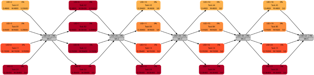
The colors in Task Block 1, 3, 4, and 5 are the same. Only in Task Block 2 where all tasks have the same amount of work (which is also the highest work a task has in this project plan), all tasks have a dark color.
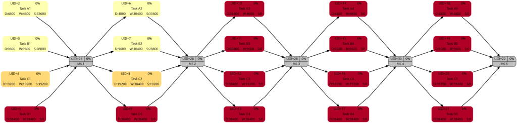
The colors in Task Block 1 and 2 are the same. The tasks in Task Blocks 3, 4, and 5 are all dark as none of these tasks has any slack.
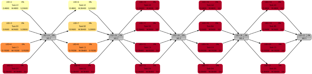
The network graph according to task criticality is similar to the one according to slack, but we can see that in Task Blocks 1 and 2 tasks get a darker color “earlier” as in the network graph according to criticality.
Example 6: Distinguishing Slack and Criticality
So far, we have not seen much difference between the network graphs according to slack and the one according to criticality. In this example, we have two task blocks with 4 tasks each where the slack is the same in the corresponding tasks in each task block. However, the duration is different between both task blocks. Work per task is almost the same, I tried to match the work despite the longer duration of the tasks in Task Block 2 as good as possible.
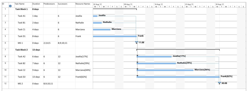
Parsing this project plan with msp2mysql.sh leads to:
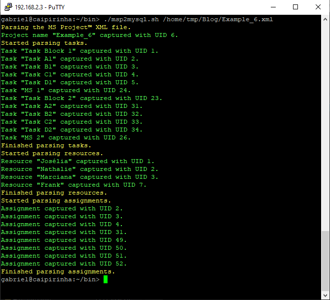
Let us look at the 4 graphs from this example:
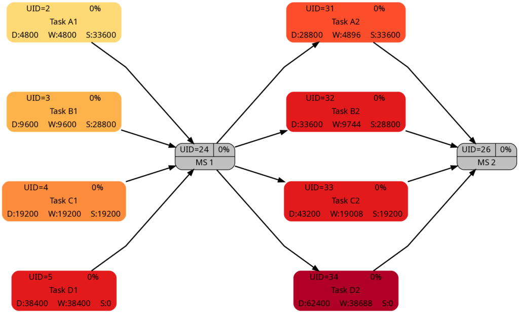
The duration of the tasks in Task Block 2 is +5d higher as in Task Block 1. Therefore, it is not surprising that the tasks in Task Block 2 are colored in darker colors.
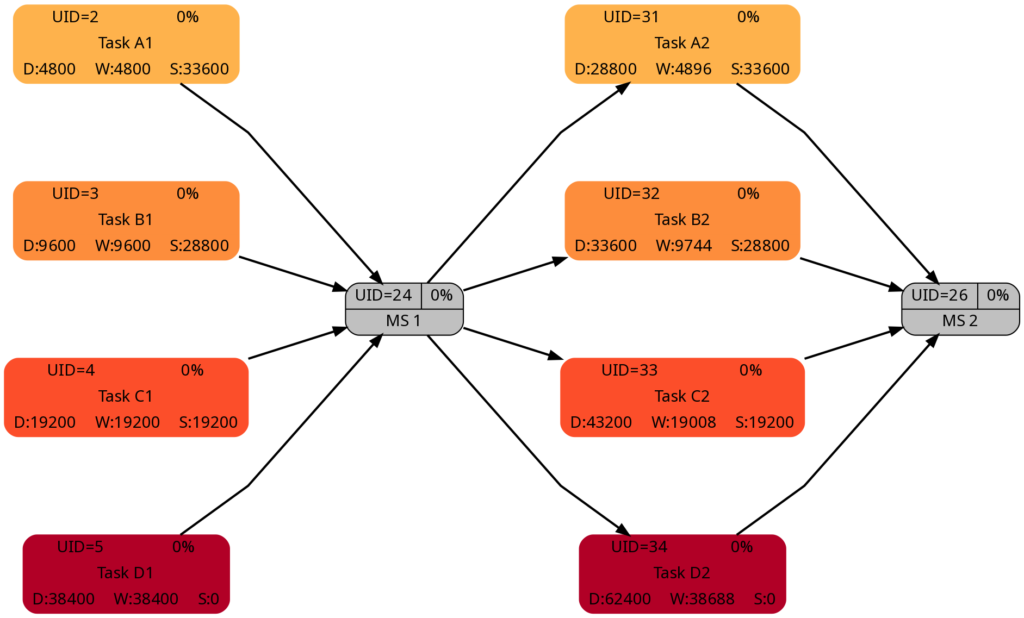
As mentioned above, I tried to keep the amount of the work the same for corresponding tasks in Task Block 1 and 2 (which can also be seen in the numeric values for the work), and consequently, the colors of corresponding tasks match.
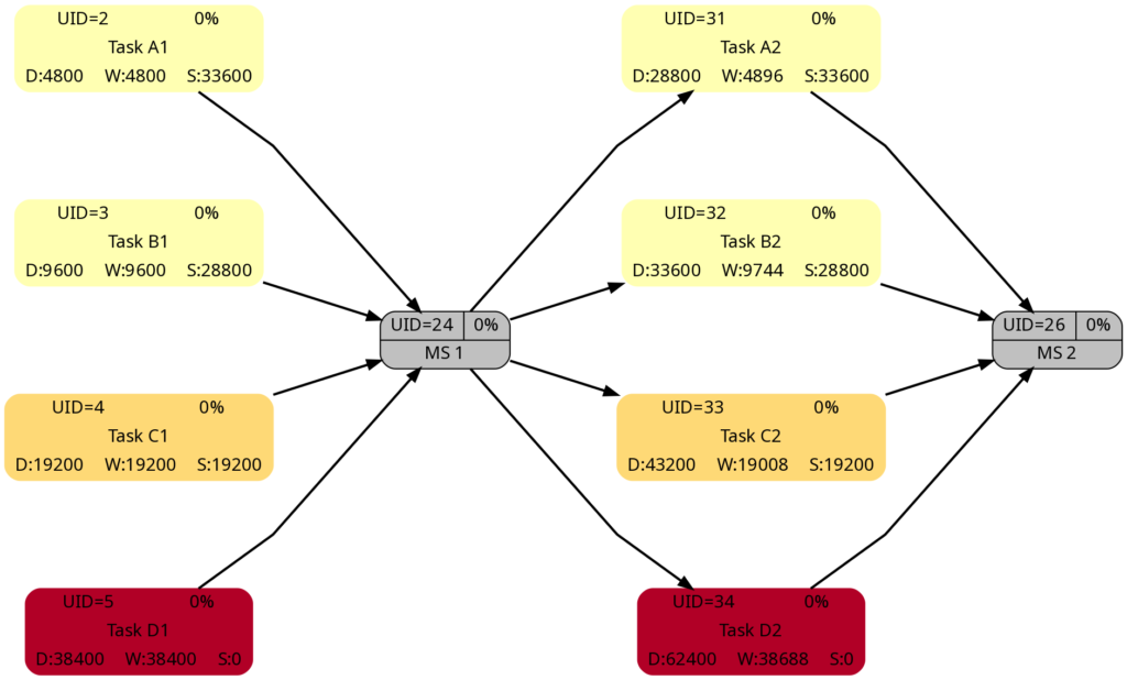
The slack of corresponding tasks in Task Block 1 and 2 is the same as the numeric values how. And so are the colors.
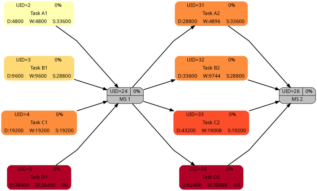
Despite the same slack of corresponding tasks in Task Block 1 and 2, the algorithm rates the criticality of the tasks in Task Block 2 higher as in Task Block 1. This is because the computation of “criticality” is based on the ratio of slack and duration. Out of two tasks with the same slack, the one with a longer duration is rated more critical as relative deviations in the duration have a higher probability to consume the free slack.
Example 7: A real-world example
Let us now look at a real-world example, a simplified project plan of a development project consisting of mechanical parts, PCBAs and software, including some intermediate milestones. As it is the case in reality, some tasks have only a partial allocation of resources, that means, that the numerical values for the allocated work are less than for the allocated duration. This will be reflected in different shadings of colors in the network graphs task duration and task duration.
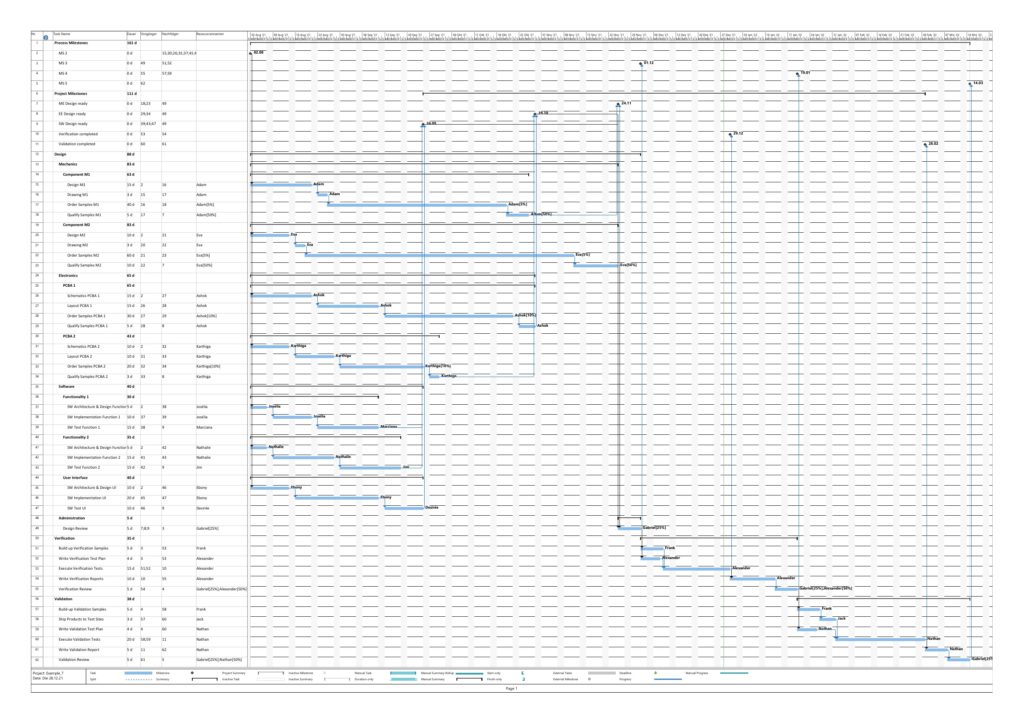
The resulting graphs are:
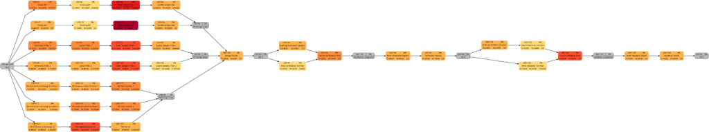
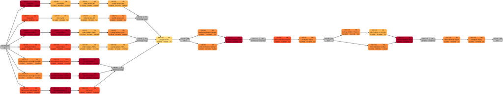
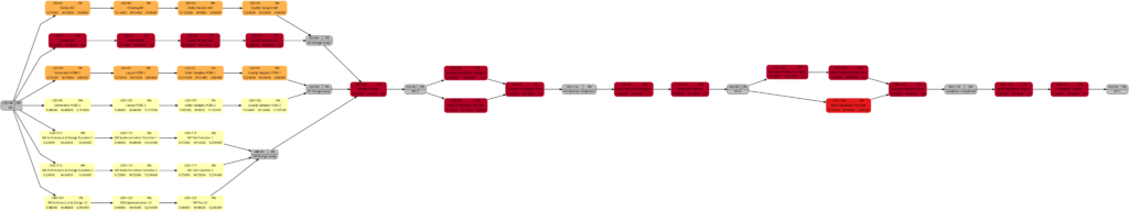
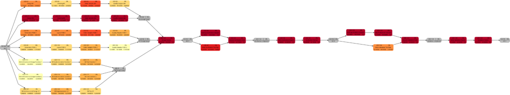
As mentioned above already, we can see the differences in the shading of the graphs according to task duration and task work, the reason being an allocation of resources different to 100%. However, in contrast to an initial expectation, the different shadings occur in large parts of the graph rather than only on a few tasks. This is because the shadings depend on the maximum and the minimum values of task duration or task work, and these values are unique to each type of graph. Well visible is also the critical path in dark red color in the network graph colored according to task criticality.
Example 8: A real-world example with complete tasks
Once a project has been started, sooner or later, the first tasks will be completed, and in this example, we assume that we have run three weeks into the project (green vertical line), and all tasks have been executed according to schedule (this is an example from an ideal world 😀). Consequently, our plan looks like this:
Tasks that have been completed 100% are colored in green color across all network graphs indicating that these tasks do not require any more attention in the remaining project:
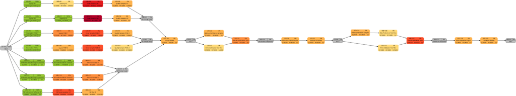
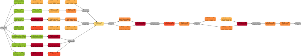
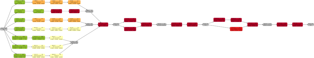
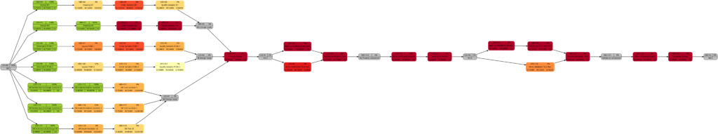
The color shadings of the incomplete tasks remain as they were in Example 7. This is because the script mysql2dot.sh determines the step size of the shadings (and thus the resulting shadings) of the individual tasks based on the maximum and minimum value of task duration, task work, task slack, or task criticality for the whole project, independent whether some tasks have been completed or not.
Conclusion
The scripts create_project_db.sql, msp2mysql.sh and mysql2dot.sh and the examples provided above show how, using the powerful graphviz package, traditional project plans created with Microsoft® Project can be visualized in a set pf graphs that can help a project manager to focus on the right tasks. For the ease of understanding, the scripts run in bash so that everyone can easily modify, enlarge, or change the scripts according to the own demands. Users who want to deploy the scripts on productive systems should take speed of execution and cybersecurity (or the lack of both in the provided example scripts) into account.
Outlook
The provided scripts can be enlarged in their scope or improved in numerous ways, and I encourage everyone to tailor them to your own needs. Some examples for improvement are:
- Improve the parsing of Microsoft® Project XML files by:
- …using a real XML parser rather than bash commands
- …enlarging the scope of the parser
- Create additional graphs.
- Consider tasks that have been completed partially.
- Experiment with different definitions of criticality.
- Explore resource usage and how to display it graphically (load, usage, key resource, etc.).
- Improve the function iso2msp () which so far is only a very simplistic implementation and is not yet able to process values like “days”, “weeks”, “months”.
Sources
- [1] = Introduction to Project XML Data
- [2] = ISO 8601 duration format
- [3] = Graphviz Color Names
- [4] = ColorBrewer License
Files
- create_project_db.sql sets up a database in MySQL or MariaDB. The script works with the user gabriel who assumes to have access to the database server without password; you might have to adapt the script to your environment and needs.
- msp2mysql.sh reads a Microsoft® Project plan in XML, parses it and writes the data into the MariaDB database.
- mysql2dot.sh reads from the MariaDB database and creates a script for dot, a tool of the graphviz suite.
- PERT-Farbskalen.xlsx is a work sheet where different approaches for color distributions are tested and where you can play around to find the “right” algorithm for yourself.
- Example_1.zip contains all files with respect to Example 1.
- Example_2.zip contains all files with respect to Example 2.
- Example_3.zip contains all files with respect to Example 3.
- Example_4.zip contains all files with respect to Example 4.
- Example_5.zip contains all files with respect to Example 5.
- Example_6.zip contains all files with respect to Example 6.
- Example_7.zip contains all files with respect to Example 7.
- Example_8.zip contains all files with respect to Example 8.
Disclaimer
- The program code and the examples are for demonstration purposes only.
- The program shall not be used in production environments.
- While the program code has been tested, it might still contain errors.
- The program code has not been optimized for speed (It’s a bash script anyway, so do not expect miracles.).
- The program code has not been written with cybersecurity aspects in mind.
- Only a subset of all possibilities in [1] has been used, and the code does not claim to adhere completely to [1].
BMW 330e (PHEV) Learnings
Since 23-Jun-2020, I have used my hybrid electric car, a BMW 330e iPerformance (F30 platform), built in 2016. I bought it from the BMW branch office in Kirkel, and I have gained quite some experience with this model since then. While some learnings may be unique to this type of car, I believe that a great deal of my experience is also applicable to other plug-in hybrid vehicles (PHEV). My experience is not applicable to electric-only cars (battery electric vehicles aka BEV).
These are the points that I would like to hightlight to someone interested in buying or using a PHEV:
General Points
Pure electric Mode (MAX eDRIVE)
- I use the purely electric mode (MAX eDRIVE) when I know that I can achieve my whole trip with the electric charge of the battery (e.g., shopping in the nearby city). When I already know that this will not be possible or when I do not yet know the extension of my whole trip, I leave the car in the default mode AUTO eDRIVE.
- I can reach a realistic maximum range of 24 km under very good conditions (no need to brake too often, summer, flat terrain). When temperatures fall, this range decreases to 15 km, and below +3°C, MAX eDRIVE does not really make sense, as the combustion engine will kick in as soon as I would accelerate only modestly.
- I get a real consumption between 0,20 kWh/km (summer time, little start-and-stop) and 0,32 kWh/km (winter time, a lot of start-and-stop). Pre-heating the car in winter would bring the consumption closer to the summer time values, but pre-heating also has a cost to it. Below are some examples of electricity consumption at various conditions.
- Driving with the electric machine in the BMW 330e is different than driving a BEV. In a BEV, you usually do not have a gearbox, and there is a fixed transmission ratio between the rotation of the electric machine and the axis. In the BMW 330e however, the electric machine is located before the gearbox, and in fact it cycles through a range of gears. In fact, even before you start to roll, the electric machine rotates with a certain idle rotation and is phased in via the clutch of the automated gearbox (ZF GA8P75HZ [1], [2]). Using the smartphone app from [3] and the ODB2 adapter from [4], I undertook some measurements in the modes Sport, Comfort, and Eco, and I found the following results:
- The switching from one gear to the next one does not seem to be related to the mode. While the “feeling” of the Sport mode is definitively more agile than the one of the Eco mode, this does not translate in earlier to later switches to the next gear when using the purely electric mode.
- During acceleration, the switch from one gear to the next higher gear seems to happen around 3000 rpm of the electric machine.
- At no load (releasing the accelerator pedal), switching down to lower gears seems to happen around these rotations:
- From 6→5: 1800 rpm
- From 5→4: 1600 rpm
- From 4→3: 1400 rpm
- From 3→2: 1300 rpm
- From 2→1: 800 rpm
Examples of electricity and fuel consumptions


Public Charging
- While things have become better, public charging can still be some kind of adventure where you can have unpleasant surprises in some cases. However, I can state that things have become much better than in the early days.
- Tariffs can vary greatly, from reasonable to outrageously expensive. One must check the tariffs at the charging station just before each recharge again, as they can change from one day to the other. Even then, this does not mean that you will also be charged the cost that is advised in the app.
- With the consumption values given above, I have set my personal limit at 0.45 €/kWh. If the tariff is higher than that, I am equally or better off if I use the combustion engine.
- Most operators will charge you additionally if your car stays longer than 3h…4h at one charging point. So be aware to stay within this duration. A few operators however have the nasty habit to charge you 0.10 €/min from the first minute on, in addition to the electricity cost. On the other side, they are a few operators that do not charge you such a penalty during the night; so you can safely start charging the car over night.
- In a large German city (Cologne), I have observed the following issue: As parking is free of charge while you are charging the car and as the parking fee on other locations is expensive, there seem to be people that connect their car on Friday evening and leave it connected at the charging point until Sunday evening. While they have to pay a penalty for exceeding the time limit (many operaters start to charge penalties after 4h), the penalty is often capped at around 12 € and therefore still much cheapter than paying for the parking fee that would otherwise have to be paid. Therefore, too, it might be difficult to find a free charging station in the center of the city.

Links
Financial Risk and Opportunity Calculation
Executive Summary
This blog post offers a method to evaluate n-ary project risks and opportunities from a probabilistic viewpoint. The result of the algorithm that will be discussed, allows to answer questions like:
- What is the probability that the overall damage resulting from incurred risks and opportunities exceeds the value x?
- What is the probability that the overall damage resulting from incurred risks and opportunities exceeds the expected value (computed as ∑(pi * vi) for all risks and opportunities)?
- How much management reserve should I assume if the management reserve shall be sufficient with a probability of y%?
The blog post shall also encourage all affected staff to consider more realistic n-ary risks and opportunities rather than the typically used binary risks and opportunities in the corporate world.
This blog post builds on the previous blog post Financial Risk Calculation and improves the algorithm by:
- removing some constraints and errors of the C code
- enabling the code to process risks and opportunities together
Introduction
In the last decades, it has become increasingly popular to not only consider project risks, but also opportunities that may come along with projects. [1] and [2] show aspects of the underlying theory, for example.
In order to accommodate that trend (and also in order to use the algorithm I developed earlier in my professional work), it became necessary to overhaul the algorithm so that it can be used with larger input vectors of risks as well as with opportunities. The current version of the algorithm (faltung4.c) does that.
Examples
Example 1: Typical Risks and Opportunities
In the first example, we will consider some typical risks and opportunities that might occur in a project. The source data for this example is available for download in the file Risks_Opportunities.xlsx.
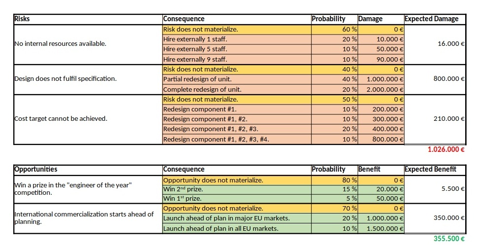
We can see a ternary, a quaternary, and a quinary risk and two ternary opportunities. This is already different from the typical corporate environment in which risks and opportunities are still mostly perceived as binary options (“will not happen” / “will happen”), probably because of a lack of methods to process any other form. At that point I would like to encourage everyone in a corporate environment to take a moment and think whether binary risks only are really still contemporary in the complex business world of today. I believe that they are not.
As already described in the previous blog post Financial Risk Calculation, these values have to copied to a structured format in order to be processed with the convolution algorithm. For the risks and the opportunities shown in the table above, that would turn out to be:
# Distribution of the Monetary Risks and Opportunities
# Risks have positive values indicating the damage values.
# Opportunities have negative values indicating the benefit values.

# START
     0    0.60
 10000    0.20
 50000    0.10
 90000    0.10
# STOP

# START
       0  0.40
 1000000  0.40
 2000000  0.20
# STOP

# START
      0   0.50
 200000   0.10
 300000   0.10
 400000   0.20
 800000   0.10
# STOP

# START
       0   0.80
  -20000   0.15
  -50000   0.05
# STOP

# START
       0   0.70
-1000000   0.20
-1500000   0.10
# STOP
Note that risks do have positive (damage) values whereas opportunities have negative (benefit) values. That is inherently programmed into the algorithm, but of course, could be changed in the C code (for those who like it the opposite way).
After processing the input with:
cat risks_opportunities_input.dat | ./faltung4.exe > risks_opportunities_output.datthe result is stored in the file risks_opportunities_output.dat which is lengthy and therefore not shown in full here on this page. However, let’s discuss about some important result values at the edge of the spectrum:
# Convolution Batch Processing Utility (only for demonstration purposes)
# The resulting probability density vector is of size: 292
# START
  -1550000   0.0006000000506639
...
   2890000   0.0011200000476837
# STOP

# The probability values are:
  -1550000   0.0006000000506639
  -1540000   0.0008000000625849
...
         0   0.2721000205919151
...
   2870000   0.9988800632822523
   2890000   1.0000000633299360
The most negative outcome corresponds to the possibility that no risk occurs, but that all opportunities realize with their best value. In our case this value is 1,550,000 €, and from the corresponding line in the density vector we see that the probability of this occurring is only 0.06%.
The most positive outcome corresponds to the possibility that no opportunity occurs and that all risks realize with their worst value. On our case, this is 2,890,000 €, and the probability of this to occur is 0.11%. In between those extreme values, there are 290 more possible outcomes (292 in total) for a benefit or damage.
Note that the probability density vector is enclosed in the tags #START and #STOP so that it can directly be used as input for another run of the algorithm.
The second part of the output contains the probability vector which (of course) also has 292 in this example. The probability vector is the integration of the probability density vector and sums up all probabilities. The first possible outcome (most negative value) therefore starts with the same probability value, but the last possible outcome (most positive value) has the probability 1. In our case, the probability is slightly higher as 1, and this is due to the fact that float or double variables in C do not have infinite resolution. In fact, already when converting a number with decimals to a float or double value, you most probably encounter imprecisions (unless the value is a multiple or fraction of 2).
The file Risks_Opportunities.xlsx contains the input vector and the output of the convolution as well as some graphic visualizations in Excel. However, for large output values, I do not recommend to process or visualize them in Excel, but instead, I recommend to use gnuplot for the visualization. The images below show the probability density distribution as well as (1 – probability distribution) as graphs generated with gnuplot.
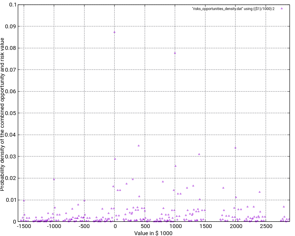
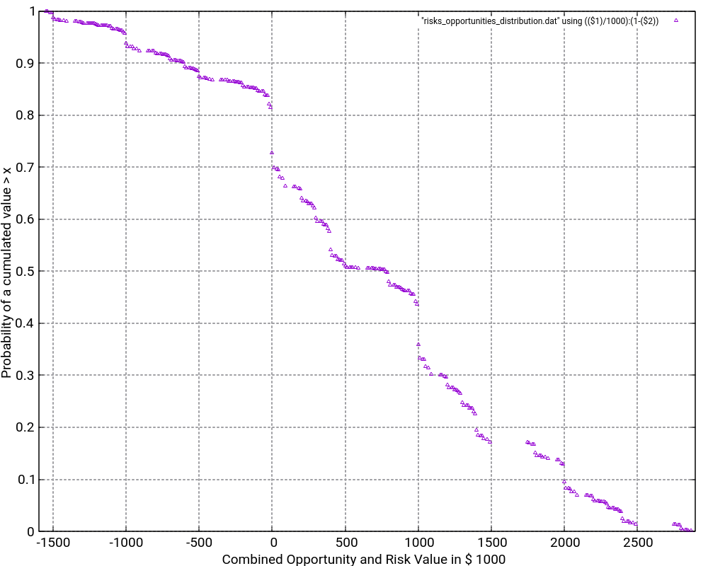
What is the purpose of the (1 – Probability distribution) graph? The purpose is to answer the question: “What is the probability that the damage value is higher as x?”
Let’s look what the probability of a damage value of more than 1,000,000 € is? In order to do so, we locate “1000” on the x-axis and go vertically up until we reach the graph. Then, we branch to the left and read the corresponding value on the y-axis. In our case, that would be something like 36%. This means that there is a probability of 36% that thus project experiences a damage of more than 1,000,000 €. This is quite a notable risk, something which one would probably not guess by just looking at the expected damage value of 1,026,000 € listed in the Excel table.
And even damage values of more than 2,000,000 € can still occur with some 10% of probability.
The graph would always start relatively on the top left and finish on the bottom right. Note that the graph does not start at 1.0 because there is a small chance that the most negative value (no risks, but the maximum of the opportunities realized) happens. However, the graph reaches the x-axis at the most positive value. Therefore, it is important asking the question “What is the probability that the damage value is higher than x?” rather than asking the question “What is the probability that the damage value is than x or higher?” The second question is incorrect although the difference might be minimal when many risks and opportunities are used as input.
Example 2: Many binary risks and opportunities of the same value
This example is not a real one, but it shall help us to understand the theory behind the algorithm. In this example, we have 200 binary risks and 200 binary opportunities with a damage or benefit value of 1,000 € and a probability of occurrence of 50%.
# Risks have positive values indicating the damage values.
# Opportunities have negative values indicating the benefit values.

# START
    0   0.50
 1000   0.50
# STOP

# START
    0   0.50
-1000   0.50
# STOP
...
From this, we can already conclude that the outcomes are in the range [-200,000 €; +200,000 €] corresponding to the rare events “no risk materializes, but all opportunities materialize” respectively “no opportunity materializes, but all risks materialize”. As the example is simple in nature, we can also conclude immediately that the possibility of such an extreme outcome is
p = 0.5(200+200) = 3.87259*10-121
and that is really a very low probability. We might also guess that the outcome value zero would have a relatively high probability as we can expect this value to be reached by many different combinations of risks and opportunities.
When we look at the resulting probability density curve and the resulting probability distribution, we can see a bell-shaped curve in the probability density and the resulting S curve as the integration of the bell-shaped curve. While the curve resembles a Gaussian distribution, this is not the case in reality as our possible outcomes are bound by a lower negative value and an upper positive value whereas a strict Gaussian distribution has a probability (and be it minimal only) for any value on the x-axis.
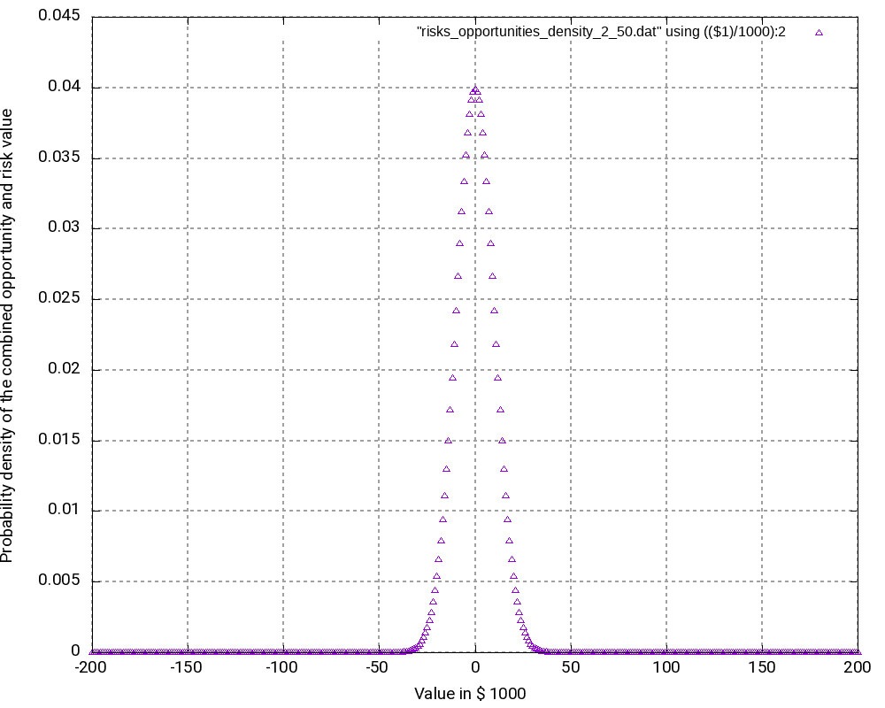
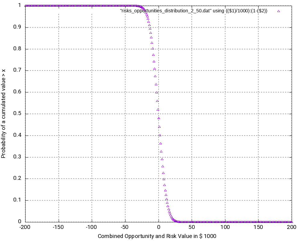
Let us have a closer look at some values in the output tables:
# Convolution Batch Processing Utility (only for demonstration purposes)
# The resulting probability density vector is of size: 401
# START
   -200000   0.0000000000000000
   -199000   0.0000000000000000
...
     -2000   0.0390817747440756
     -1000   0.0396709472276547
         0   0.0398693019637929
      1000   0.0396709472276547
      2000   0.0390817747440756
...
    199000   0.0000000000000000
    200000   0.0000000000000000
# STOP

# The probability values are:
   -200000   0.0000000000000000
   -199000   0.0000000000000000
...
     -2000   0.4403944017904490
     -1000   0.4800653490181037
         0   0.5199346509818966
      1000   0.5596055982095512
      2000   0.5986873729536268
...
    199000   0.9999999999999996
    200000   0.9999999999999996
The following observations can be made:
- The most negative outcome (-200,000 €) and the most positive outcome (+200,000 €) can only be reached in one constellation and have, as calculated above, minimal probability of occurrence. Therefore, the probability density vector shows all zero in the probability.
- The outcome 0 has the highest probability of all possible outcomes (3.99%), and outcomes close to 0 have a similarly high probability. Hence, it is very probable that the overall outcome of a project with this (artificially constructed) risk and opportunity pattern is around 0.
- It may astonish at first that in the probability distribution (not the probability density), the value 0 is attributed to a probability of 51.99% rather than to 50.00%. However, we must keep in mind that the values in the probability distribution answer the question: “What is the probability that the outcome is > x?” and not “… ≥ x?” That makes the difference.
- At the upper end of the probability distribution (+200,000 €), we would expect the probability to be 1.0 rather than a value below that. However, here, the limited resolution of even double variables in C result in the fact that errors in the precision of arithmetic results add up. This might be improved by using long double as probability variable.
Example 3
The third example is similar to the second one, but it only contains risks, that is, we leave away all opportunities from the second example. Consequently, outcomes (damages) lie in the interval [0; +200,000 €]. The outcomes at the edges of the interval have the lowest probability of occurrence, in this case:
p = 0.5200 = 6.22302*10-61
While this probability of occurrence is much higher than the one for the edge values in Example 2, it is still very low.
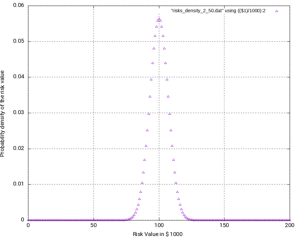
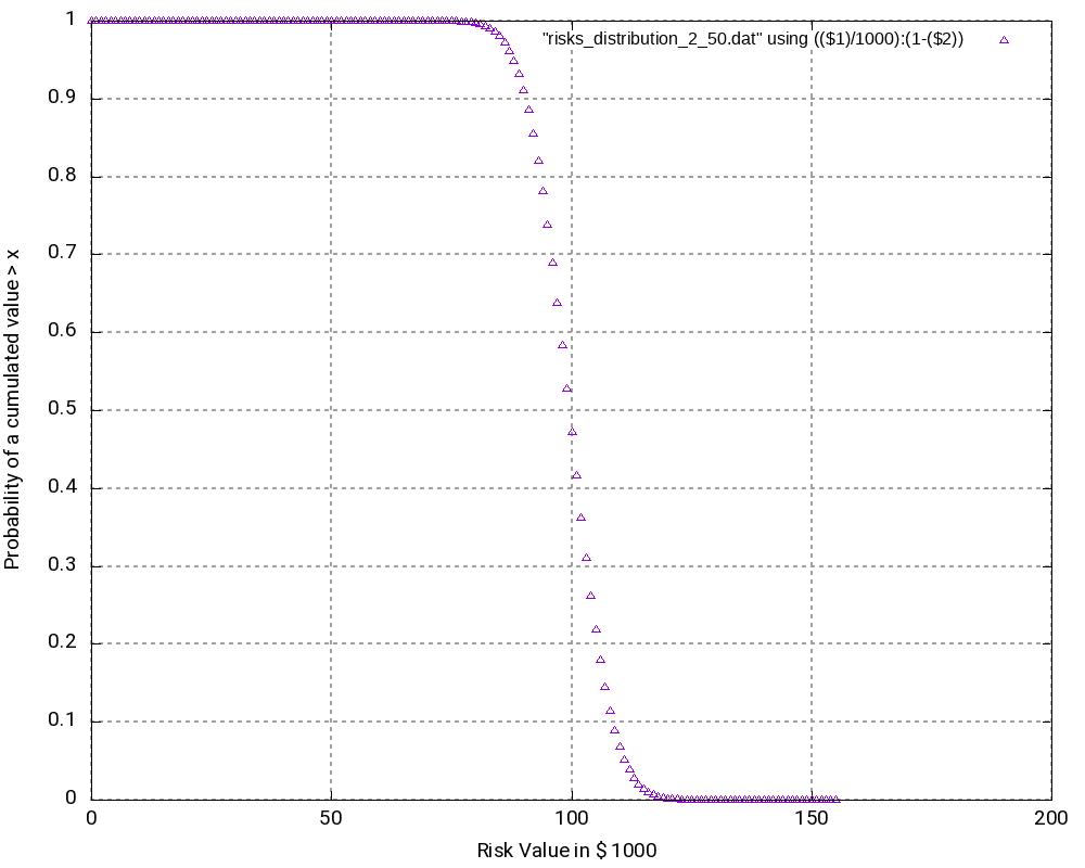
As we can see (and this could be expected somewhat), the most probably outcome now is a damage of +100,000 €, again the value in the middle of the interval which now has a probability of occurrence of 5.63% (higher than in the second example). While the curves in the second and in the third example look very similar, the curves are “steeper” in the third example.
# Convolution Batch Processing Utility (only for demonstration purposes)
# The resulting probability density vector is of size: 201
# START
         0   0.0000000000000000
      1000   0.0000000000000000
...
     99000   0.0557905732764915
    100000   0.0563484790092564
    101000   0.0557905732764915
...
    199000   0.0000000000000000
    200000   0.0000000000000000
# STOP

# The probability values are:
         0   0.0000000000000000
      1000   0.0000000000000000
...
     99000   0.4718257604953718
    100000   0.5281742395046283
    101000   0.5839648127811198
...
    199000   1.0000000000000002
    200000   1.0000000000000002
Conclusion
This blog post shows that with the help of the algorithm faltung4.c, it has become possible to computer probability densities and probability distributions of combined risks and opportunities and answer valid and important questions with respect to the project risk and the monetary reserves (aka “management reserve”) that should be attributed to a project with a certain portfolio of risks and opportunities.
Outlook
The algorithm may be enlarged so that it can accommodate start and finish dates of risks and opportunities. In this case, probability densities and probability distributions can be computed for any point in time that changes the portfolio of risks and opportunities due to the start or finish of a risk or opportunity. In this case, the graphs will become 3-dimensional and look somewhat like a “mountain area”. This would have relevance in the sense that some projects might start heavily on the risky side and opportunities might only become available later. For such projects, there is a real chance that materialized risks result in a large cash outflow which later is then partially compensated by materialized opportunities.
Sources
- [1] = Balancing project risks and opportunities
- [2] = Project opportunity – risk sink or risk source?
Files
- Risks_Opportunities.xlsx contains the example table as well as the result tables of the analysis, graphs and some scripting commands.
- faltung4.c contains the C program code that was used for the analysis.
- Example 1:
- risks_opportunities_input.dat is the input table.
- risks_opportunities_output.dat is the output table which contains the probability density and the probability distribution.
- risks_opportunities_density.dat is the output table containing the probability density only.
- risks_opportunities_density.png is a graphic visualization of the probability density with gnuplot.
- risks_opportunities_distribution.dat is the output table containing the probability distribution only.
- risks_opportunities_distribution.png is a graphic visualization of (1 – probability distribution) with gnuplot.
- Example 2:
- risks_opportunities_input_2_50.dat is the input table.
- risks_opportunities_output_2_50.dat is the output table which contains the probability density and the probability distribution.
- risks_opportunities_density_2_50.dat is the output table containing the probability density only.
- risks_opportunities_density_2_50.png is a graphic visualization of the probability density with gnuplot.
- risks_opportunities_distribution_2_50.dat is the output table containing the probability distribution only.
- risks_opportunities_distribution_2_50.png is a graphic visualization of (1 – probability distribution) with gnuplot.
- Example 3:
- risks_input_2_50.dat is the input table.
- risks_output_2_50.dat is the output table which contains the probability density and the probability distribution.
- risks_density_2_50.dat is the output table containing the probability density only.
- risks_density_2_50.png is a graphic visualization of the probability density with gnuplot.
- risks_distribution_2_50.dat is the output table containing the probability distribution only.
- risks_distribution_2_50.png is a graphic visualization of (1 – probability distribution) with gnuplot.
Usage
Scripts and sequences indicating how to use the algorithm faltung4.c can be found in the table Risks_Opportunities.xlsx on the tab Commands and Scripts. Please follow these important points:
- The input file which represents n-ary risks and n-ary opportunities as well as their probabilities of occurrence, has to follow a certain structure which is hard-coded in the algorithm faltung4.c. A risk or opportunity is always enclosed in the tags # START and # STOP.
- Lines starting with “#” are ignored as are empty lines.
- The probabilities of occurrence of an n-ary risk or an n-ary opportunity must sum up to 1.0.
- The C code can be compiled with a standard C compiler, e.g., gcc, with the sequence:
gcc -o faltung4.exe faltung4.c- The input file is computed and transformed into an output file with the sequence:
cat input_file.dat | ./faltung4.exe > output_file.dat- The output file consists of two parts:
- a resulting probability density which has the same structure as the input file (with the tags # START and # STOP)
- a resulting probability distribution
- In order to post-process the output, e.g., with gnuplot, you can help yourself with standard Unix tools like head, tail, wc, cat, etc.
- The output file is structured in a way so that it can be easily used for visualizations with gnuplot.
Disclaimer
- The program code and the examples are for demonstration purposes only.
- The program shall not be used in production environments.
- While the program code has been tested, it might still contain errors.
- Due to rounding errors with float variables, you might experience errors depending on your input probability values when reading the input vector.
- The program code has not been optimized for speed.
- The program code has not been written with cybersecurity aspects in mind.
- This method of risk and opportunity assessment does not consider that risks and opportunities in projects might have different life times during the project, but assumes a view “over the whole project”. In the extreme case, for example, that risks are centered at the beginning and opportunities are centered versus the end of a project, it might well be possible that the expected damage/benefit of the overall project is significantly exceeded or significantly subceeded.
DICOM Experiments with dcmtk and TLS
Executive Summary
In this small article, I would like to point out how we can use the command line tools from the dcmtk toolkit in order to play around with DICOM images, setting up a DICOM recipient and how we integrate TLS (encryption) in the whole setup.
The dcmtk toolkit is a powerful set of command line tools which enable us to play around with DICOM, program test environments, transform images between DICOM and other common formats (like JPEG or PNG) and simulate a simple PACS or a worklist server. It does not feature all tools that you would wish to have (e.g., dealing with MP4 videos), but it’s powerful enough to start with.
As always, I recommend that you execute all scripts on a properly installed Linux machine. (Windows will also do it, but it’s… uh!) Fortunately, the dcmtk toolkit is available for most Linuxes.
Sending DICOM images
Let’s start with a simple setup. We need a folder structure like this:
gabriel@caipirinha:~> tree /reserve/playground/
/reserve/playground/
├── images
│   ├── IM000001
│   ├── IM000002
│   ├── IM000003
│   ├── IM000004
│   ├── IM000005
│   ├── IM000006
│   ├── IM000007
│   ├── IM000008
│   └── IM000009
└── pacs
The folder images will contain some sample DICOM images. Either you have some from your own medical examinations, or you download some demo pictures from the web. The folder pacs will serve as recipient of our transmitted DICOM images.
We furthermore need two (bash) shells open, and in the first shell, we start a storescp instance:
storescp +B +xa -dhl -uf -aet PACS -od /reserve/playground/pacs 10400
This command enables a recipient of DICOM images; it will be our “mini” PACS, and it will just store all the data it receives in the folder /reserve/playground/pacs.
The storescp command has a range of options which you might explore using “man storescp” on your Linux machine. Here, we use the options:
- +B: write data exactly as read. Actually, I use this option as it seems to write directly on disk. On a weaker Raspberry Pi I did have issues with large files until I started to use this option. So: recommended.
- +xa: accept all supported transfer syntaxes. That’s what you expect from a test system.
- -dhl: disable hostname lookup. In our test environment, we do not want to complicate things by using DNS and reverse DNS lookups.
- -uf: generate filename from instance UID (default). This means that you will get files names from the instance UID. They are not exactly “telling” filenames, but they refer to some instance UID that comes from your other test systems or from a worklist or from whereever.
- -aet: set my AE title. This is the AE title, an important identifier in the DICOM world. In reality, this would probably be a name referring to the respective hospital owning the PACS or to the manufacturer of the PACS.
You can also see that the instance is listening on TCP port 10400. This is not the standardized port for DICOM operation; in fact, in reality you would use port 104. But as we want to test around not using the root account, we will not use privileged ports.
In the second shell, we transmit a DICOM image by invoking a storescu command:
storescu localhost 10400 /reserve/playground/images/IM000001
This will transfer the DICOM image IM000001 to the storescp and ultimately store it in the folder /reserve/playground/pacs. The whole operation looks like in the image below. Do not get bothered by the messages of the storescu command; it just evidences that even commercially taken DICOM images do not always fulfil the specs.
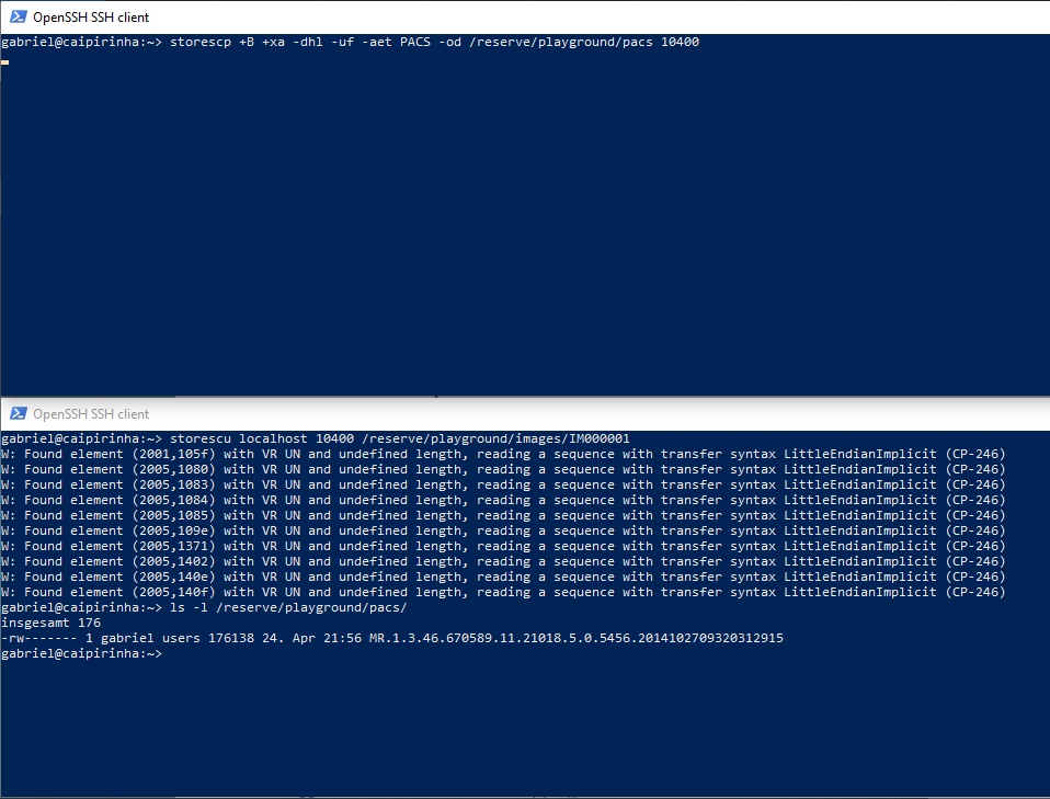
Sending DICOM images with TLS
Now, let’s switch one gear higher and use TLS encryption for the transfer of our DICOM image. We need some preparation though, and for that, we need to download a script named dcmtk_ca.pl. You can get that at Github, for example (here). Save it and make it executable. Of course, you need a Perl interpreter, but as you work on a well installed Linux machine, it is simply available.
We first need to create a (self-generated) root certificate and subsequently two key pairs. On this blog post, you can find the commands for that, and those are:
./dcmtk_ca.pl newca /reserve/playground/myca
mkdir /reserve/playground/mycert
./dcmtk_ca.pl mkcert -des no /reserve/playground/myca/ /reserve/playground/mycert/cert1 /reserve/playground/mycert/key1
./dcmtk_ca.pl mkcert -des no /reserve/playground/myca/ /reserve/playground/mycert/cert2 /reserve/playground/mycert/key2
During the course of the execution of these commands, you will be asked several questions which refer to attributes used in X.509 certificates, like “organizational unit”, … The values that you give do not matter here in our test environment. But for certificates used in production environment, those attributes should be populated with meaningful values, of course.
The command sequence above has created our root certificate in the file /reserve/playground/myca/cacert.pem, and two key pairs in the folder /reserve/playground/mycert/. We will now repeat the transmission of a DICOM image as shown in the previous chapter, however, using a TLS connection. Hence, in our first shell, we will issue the command:
storescp +B +xa -dhl -uf --aetitle PACS -od /reserve/playground/pacs +tls /reserve/playground/mycert/key1 /reserve/playground/mycert/cert1 --add-cert-file /reserve/playground/myca/cacert.pem 2762
which will be our “mini” PACS again, and in the second shell we issue the command:
storescu +tls /reserve/playground/mycert/key2 /reserve/playground/mycert/cert2 --add-cert-file /reserve/playground/myca/cacert.pem localhost 2762 /reserve/playground/images/IM000001
You can see that for this example, I have used TCP port 2762 which is also the recommendation from NEMA.
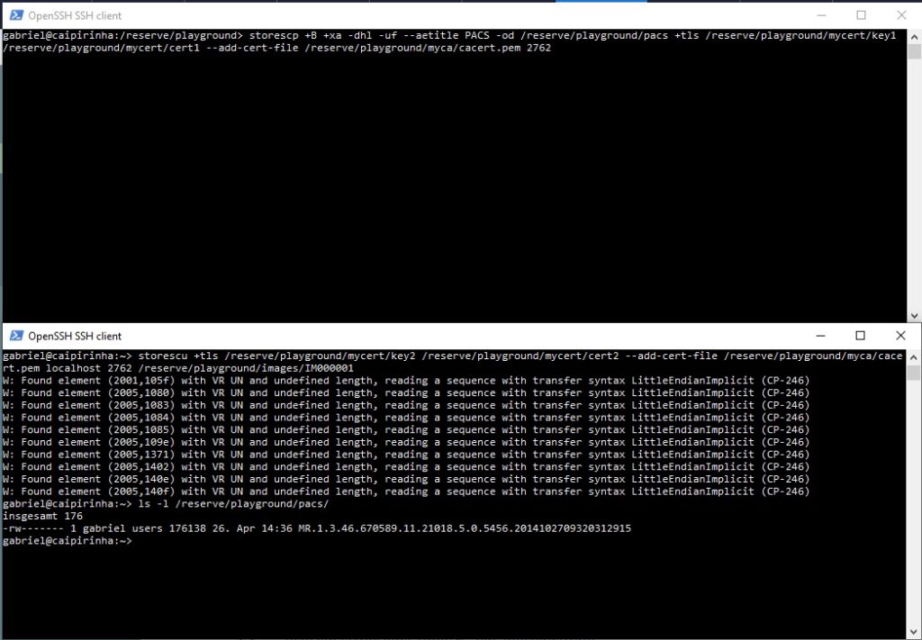
In this example, we have used a self-generated root certificate (cacert.pem) and derived two key pairs from this. But in real life, you might have an existing certificate that shall be used. My web server (caipirinha.spdns.org) for example, has a real certificate (thanks to the Let’s Encrypt initiative), and now, we want to use this certificate for the storescp sequence simulating our “mini” PACS. In order to do so, I will start the storescp instance as root user (because on my machine, only root can read the server key). On a production system, this is exactly what you shall not do; rather than that, you will have to find a way for you to make the server key available for the user which shall run the PACS, and this user should not be a normal user. But for our test here, this is OK. So, in that case, the storescp command would be:
storescp +B +xa -dhl -uf --aetitle PACS -od /reserve/playground/pacs +tls /etc/letsencrypt/live/caipirinha.spdns.org/privkey.pem /etc/letsencrypt/live/caipirinha.spdns.org/cert.pem +cf /reserve/playground/myca/cacert.pem 2762
The corresponding storescu command is:
storescu +tls /reserve/playground/mycert/key2 /reserve/playground/mycert/cert2 --add-cert-file /reserve/playground/caipirinha-spdns-org-zertifikatskette.pem localhost 2762 /reserve/playground/images/IM000001
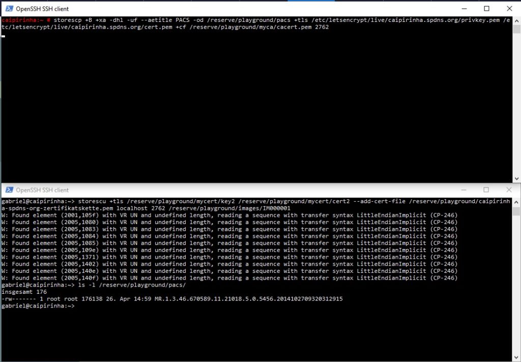
You will realize here that in this example, the storescp instance has the root certificate of the storescu instance (which is the self-generated root certificate) whereas the storescu instance has the root ceritifcate chain of the storescp instance (which I extracted using the Firefox browser and accessing my own page https://caipirinha.spdns.org/). The reason for this crossover mentioning of the root certificates is simple:
- The storescp instance needs the root certificate (chain) of the storescu instance in order to verify whether the certificate that the storescu instance presents is valid.
- The storescu instance needs to the root certificate (chain) of the storescp instance in order to verify whether the certificate that the storescp instance presents is valid.
This might put a problem for hospital installations. Very rarely would you be able to add self-generated root certificates to your PACS, and therefore, the recommendation is that, when using TLS in your hospital environment, the probably best approach is that all certificates (key pairs) are generated from the very same certificate authority that was used to issue the key pair for the PACS. How certificate and key information is set up in various DICOM-capable devices depend on the device. In one device I came across, all related certificates and keys could be saved on the hard disk where I created a folder D:\Zertifikate and subsequently entered the related information in a JSON object for the DICOM configuration. That looked like this:
{
 ...
 "DefaultSendOptions": {
    "sendExecutable": "storescu-tls.exe",
    ...
    },
    "args": [
      "--log-level",
      "info",
      ...
      "+tls",
      "D:/Zertifikate/key",
      "D:/Zertifikate/cert",
      "+cf",
      "D:/Zertifikate/caipirinha-ca-chain.pem"
    ],
    ...
}
In this example, I still used a self-created certificate and key for the DICOM-enabled device that shall talk to the PACS, but the PACS itself uses a real certificate. You can see that the DICOM-enabled device also uses the storescu command in order to transmit DICOM data. This is not unusual, as most device manufacturers would use the dcmtk toolkit rather than programming DICOM routines from scratch.
I hope that this small article can help you to better understand the two related commands storescp and storescu with the focus on TLS encryption during the communication.
Links
Key Words
USV
Konzept
Die Stabilität eines Servers hängt auch von der Versorgungssicherheit des Stromnetzes ab. Hier drohen folgende Gefahren:
- Stromausfall
- Spannungsschwankungen
- Blitzschlag bzw. plötzliche Überspannung
Diese Ursachen können plötzlichen Systemabsturz oder gar Hardware-Schäden zur Folge haben und müssen daher vermieden werden. Glücklicherweise wird man mit solchen Problemen in Deutschland weniger geplagt als in weniger entwickelten Ländern, wo solche Probleme im wörtlichen Sinne an der Tagesordnung sind.
Um dennoch Risiken zu minimieren, ist der Caipirinha-Server nicht direkt ans Stromnetz angeschlossen, sondern er wird über eine “unterbrechungsfreie Stromversorgung” (USV) betrieben. Die Wahl fiel auf eine kleine SoHo-Version der Herstellers APC, in diesem Fall das Modell “BE700-GR“, weil diese preiswert zu bekommen war und über den USB-Anschluß mit dem Server verbunden werden kann. Sie bietet außerdem Blitzschutz (im üblichen Rahmen) für sie Stromversorgung und für eine durchgeschleifte Datenleitung, was hier für die DSL-Leitung benutzt wird.
Am Standort des Caipirinha-Servers ist daher nicht nur der Server selbst an die USV angeschlossen, sondern auch der WLAN-Router und die Telefone, so dass bei einem kurzfristigen Stromausfall keine Beeinträchtigung des WLANs oder des Telefonnetzes oder des Serverbetriebs auftritt.
Einrichtung
Bei openSuSE-Linux gibt es glücklicherweise gleich ein ganzes Paket zur Kommunikation des Servers mit einer USV von APC. Dazu muss man das Paket apcupsd installieren. Nach der Installation befinden sich auf dem Server mehrere Programme, von denen der gleichnamige Dämon (apcupsd) das wichtigste ist. Dieser Dämon überwacht den Zustand der USV und kann in Abhängigkeit von gezielt diesem verschiedene Aktionen auslösen. Die zentrale Konfigurationsdatei ist /etc/apcupsd/apcupsd.conf. Die Default-Datei ist ausreichend kommentiert, so dass man sich gut darin zurechtfinden kann. Auf [1] gibt es außerdem eine sehr ausführliche und gut verständliche Dokumentation. Hier ist die aktuelle Konfiguration des Caipirinha-Servers abgedruckt:
## apcupsd.conf v1.1 ##
#
#  for apcupsd release 3.12.1 (06 January 2006) - suse
#
# "apcupsd" POSIX config file

#
# ========= General configuration parameters ============
#

# UPSNAME xxx
#   Use this to give your UPS a name in log files and such. This
#   is particulary useful if you have multiple UPSes. This does not
#   set the EEPROM. It should be 8 characters or less.
UPSNAME APC ES 700

# UPSCABLE <cable>
#   Defines the type of cable connecting the UPS to your computer.
#
#   Possible generic choices for <cable> are:
#     simple, smart, ether, usb
#
#   Or a specific cable model number may be used:
#     940-0119A, 940-0127A, 940-0128A, 940-0020B,
#     940-0020C, 940-0023A, 940-0024B, 940-0024C,
#     940-1524C, 940-0024G, 940-0095A, 940-0095B,
#     940-0095C, M-04-02-2000
#
UPSCABLE usb

# To get apcupsd to work, in addition to defining the cable
# above, you must also define a UPSTYPE, which corresponds to
# the type of UPS you have (see the Description for more details).
# You must also specify a DEVICE, sometimes referred to as a port.
# For USB UPSes, please leave the DEVICE directive blank. For
# other UPS types, you must specify an appropriate port or address.
#
# UPSTYPE   DEVICE           Description
# apcsmart  /dev/tty**       Newer serial character device,
#                            appropriate for SmartUPS models using
#                            a serial cable (not USB).
#
# usb       <BLANK>          Most new UPSes are USB.
#                            A blank DEVICE setting enables
#                            autodetection, which is th best choice
#                            for most installations.
#
# net       hostname:port    Network link to a master apcupsd
#                            through apcupsd's Network Information
#                            Server. This is used if you don't have
#                            a UPS directly connected to your computer.
#
# snmp      hostname:port:vendor:community
#                            SNMP Network link to an SNMP-enabled
#                            UPS device. Vendor is the MIB used by
#                            the UPS device: can be "APC", "APC_NOTRAP"
#                            or "RFC" where APC is the powernet MIB,
#                            "APC_NOTRAP" is powernet with SNMP trap
#                            catching disabled, and RFC is the IETF's
#                            rfc1628 UPS-MIB. Port is usually 161.
#                            Community is "private".
#
# dumb      /dev/tty**       Old serial character device for use
#                            with simple-signaling UPSes.
#
UPSTYPE usb

# LOCKFILE <path to lockfile>
#   Path for device lock file.
LOCKFILE /var/apcupslock

#
# ======== Configuration parameters used during power failures ==========
#

# The ONBATTERYDELAY is the time in seconds from when a power failure
#   is detected until we react to it with an onbattery event.
#
#   This means that, apccontrol will be called with the powerout argument
#   immediately when a power failure is detected.  However, the
#   onbattery argument is passed to apccontrol only after the
#   ONBATTERYDELAY time.  If you don't want to be annoyed by short
#   powerfailures, make sure that apccontrol powerout does nothing
#   i.e. comment out the wall.
ONBATTERYDELAY 5

#
# Note: BATTERYLEVEL, MINUTES, and TIMEOUT work in conjunction, so
# the first that occurs will cause the initation of a shutdown.
#

# If during a power failure, the remaining battery percentage
# (as reported by the UPS) is below or equal to BATTERYLEVEL,
# apcupsd will initiate a system shutdown.
BATTERYLEVEL 10

# If during a power failure, the remaining runtime in minutes
# (as calculated internally by the UPS) is below or equal to MINUTES,
# apcupsd, will initiate a system shutdown.
MINUTES 1

# If during a power failure, the UPS has run on batteries for TIMEOUT
# many seconds or longer, apcupsd will initiate a system shutdown.
# A value of 0 disables this timer.
#
#  Note, if you have a Smart UPS, you will most likely want to disable
#    this timer by setting it to zero. That way, you UPS will continue
#    on batteries until either the % charge remaing drops to or below BATTERYLEVEL,
#    or the remaining battery runtime drops to or below MINUTES.  Of course,
#    if you are testing, setting this to 60 causes a quick system shutdown
#    if you pull the power plug.
#  If you have an older dumb UPS, you will want to set this to less than
#    the time you know you can run on batteries.
TIMEOUT 0

#  Time in seconds between annoying users to signoff prior to
#  system shutdown. 0 disables.
ANNOY 30

# Initial delay after power failure before warning users to get
# off the system.
ANNOYDELAY 30

# The condition which determines when users are prevented from
# logging in during a power failure.
# NOLOGON <string> [ disable | timeout | percent | minutes | always ]
NOLOGON disable

# If KILLDELAY is non-zero, apcupsd will continue running after a
# shutdown has been requested, and after the specified time in
# seconds attempt to kill the power. This is for use on systems
# where apcupsd cannot regain control after a shutdown.
# KILLDELAY <seconds>  0 disables
KILLDELAY 0

#
# ==== Configuration statements for Network Information Server ====
#

# NETSERVER [ on | off ] on enables, off disables the network
#  information server. If netstatus is on, a network information
#  server process will be started for serving the STATUS and
#  EVENT data over the network (used by CGI programs).
NETSERVER on

# NISIP <dotted notation ip address>
#  IP address on which NIS server will listen for incoming connections.
#  Default value is 0.0.0.0 that means any incoming request will be
#  serviced but if you want it to listen to a single subnet you can
#  set it up to that subnet address, for example 192.168.10.0
#  Additionally you can listen for a single IP like 192.168.10.1
NISIP 0.0.0.0

# NISPORT <port> default is 3551 as registered with the IANA
#  port to use for sending STATUS and EVENTS data over the network.
#  It is not used unless NETSERVER is on. If you change this port,
#  you will need to change the corresponding value in the cgi directory
#  and rebuild the cgi programs.
NISPORT 3551

# If you want the last few EVENTS to be available over the network
# by the network information server, you must define an EVENTSFILE.
EVENTSFILE /var/log/apcupsd.events

# EVENTSFILEMAX <kilobytes>
#  By default, the size of the EVENTSFILE will be not be allowed to exceed
#  10 kilobytes.  When the file grows beyond this limit, older EVENTS will
#  be removed from the beginning of the file (first in first out).  The
#  parameter EVENTSFILEMAX can be set to a different kilobyte value, or set
#  to zero to allow the EVENTSFILE to grow without limit.
EVENTSFILEMAX 30

#
# ========== Configuration statements used if sharing =============
#            a UPS and controlling it via the network

# The configuration statements below are used if you want to share one
# UPS to power multiple machines and have them communicate by the network.
# Most of these items are for Master/Slave mode only, however NETTIME is
# also used for Client/Server NIS networking with the net driver.

# NETTIME <int>
#   Interval (in seconds) at which the slave or client polls the master
#   or server. This is applicable to BOTH master/slave and client/server
#   (NIS) networking.
#NETTIME 100

#
# Remaining items are for Master/Slave networking ONLY
#

# UPSCLASS [ standalone | shareslave | sharemaster | netslave | netmaster ]
#   Normally standalone unless you share a UPS with multiple machines.
#
UPSCLASS standalone

# UPSMODE [ disable | share | net | sharenet ]
#   Unless you want to share the UPS (power multiple machines),
#   this should be disable.
UPSMODE disable

# NETPORT <int>
#   Port on which master/slave networking communicates.
#NETPORT 6666

# MASTER <machine-name>
#   IP address of the master. Only applicable on slaves.
#MASTER

# SLAVE <machine-name>
#   IP address(es) of the slave(s). Only applicable on master.
#SLAVE slave1
#SLAVE slave2

# USERMAGIC <string>
#   Magic string use by slaves to identify themselves. Only applicable
#   on slaves.
#USERMAGIC

#
# ===== Configuration statements to control apcupsd system logging ========
#

# Time interval in seconds between writing the STATUS file; 0 disables
STATTIME 0

# Location of STATUS file (written to only if STATTIME is non-zero)
STATFILE /var/log/apcupsd.status

# LOGSTATS [ on | off ] on enables, off disables
# Note! This generates a lot of output, so if
#       you turn this on, be sure that the
#       file defined in syslog.conf for LOG_NOTICE is a named pipe.
#  You probably do not want this on.
LOGSTATS off

# Time interval in seconds between writing the DATA records to
#   the log file. 0 disables.
DATATIME 0

# FACILITY defines the logging facility (class) for logging to syslog.
#          If not specified, it defaults to "daemon". This is useful
#          if you want to separate the data logged by apcupsd from other
#          programs.
#FACILITY DAEMON


Mit den Parametern BATTERYLEVEL und MINUTES kann man einstellen, ab wann der Shutdown des Servers eingeleitet wird, nämlich beim Unterschreiten der angegebenen Batterieladung oder beim Unterschreiten der voraussichtlichen Restlaufzeit. In diesem Fall leitet der apcupsd-Dämon das kontrollierte Herunterfahren des Servers ein, so dass der Server nicht plötzlich stromlos wird, wenn die Batterie leer wird. Das ist sehr praktisch, weil man so inkonsistente Daten auf Platten vermeidet, welche sonst beim Absturz einer Maschine immer mal wieder auftreten.
Der Parameter NETSERVER erlaubt nicht nur den Zugriff entfernter Maschinen auf die USV-Verwaltung des Caipirinha-Servers, sondern ist auch für das reibungslose Funktionieren der anderen Programme in der apcupsd-Suite erforderlich und sollte deshalb auf ON gesetzt werden. Wenn sich mehrere Server eines USV teilen, kann man über Port 3551 auf dem Caipirinha-Server den Zustand der USV abfragen. Dadurch wissen dann alle Server, wann sie mit dem Herunterfahren beginnen sollen.
Der Parameter ANNOY gibt die Zeitspanne an, nach der Benutzer auf dem Caipirinha-Server immer wieder durch eine Mitteilung gewarnt werden, wenn der Server im Batteriebetrieb läuft. Diese regelmäßige Warnung soll Benutzer dazu verleiten, sich möglichst umgehend von der Maschine auszuloggen. Auch Benutzer von entfernten Maschinen, die über eine textbasierte Shell auf dem Caipirinha-Server arbeiten, erhalten eine entsprechende Meldung.
Nach der Anpassung der Konfigurationsdatei sind noch folgende Schritte notwendig:
- Mit dem Befehl
mkdir /var/apcupslockerzeugt man als Benutzer root noch das Verzeichnis /var/apcupslock, damit apcupsd in diesem Verzeichnis LOCK-Dateien anlegen kann. Es ist nicht erforderlich, noch den Eigentümer zu ändern. - Nun startet man den apcupsd-Dämon mit dem Befehl
/etc/init.d apcupsd start.
Wenn der apcupsd-Dämon läuft, informiert der den Benutzer root, wenn es Unregelmäßigkeiten in der Stromversorgung gibt. Dies ist so in den Skripten der apcupsd-Suite festgelegt und muss dort geändert werden, wenn eine weitergehende Benachrichtigung gewünscht wird.
Dienstprogramme
Den Status der USV kann man mit dem Programm apcaccess (mit /usr/sbin/apcaccess auch als normaler Benutzer) auslesen. Auf dem Caipirinha-Server erhält man dann beispielsweise:
APC      : 001,037,1008
DATE     : Thu Jun 24 18:55:34 CEST 2010
HOSTNAME : caipirinha
VERSION  : 3.14.6 (16 May 2009) suse
UPSNAME  : APC ES 700
CABLE    : USB Cable
MODEL    : Back-UPS ES 700G
UPSMODE  : Stand Alone
STARTTIME: Tue Jun 15 08:09:37 CEST 2010
STATUS   : ONLINE
LINEV    : 226.0 Volts
LOADPCT  :  21.0 Percent Load Capacity
BCHARGE  : 100.0 Percent
TIMELEFT :  24.1 Minutes
MBATTCHG : 15 Percent
MINTIMEL : 1 Minutes
MAXTIME  : 0 Seconds
SENSE    : Medium
LOTRANS  : 180.0 Volts
HITRANS  : 266.0 Volts
ALARMDEL : Always
BATTV    : 13.7 Volts
LASTXFER : Unacceptable line voltage changes
NUMXFERS : 2
XONBATT  : Thu Jun 24 09:39:40 CEST 2010
TONBATT  : 0 seconds
CUMONBATT: 12 seconds
XOFFBATT : Thu Jun 24 09:39:42 CEST 2010
LASTSTEST: Sat Jun 19 12:17:27 CEST 2010
STATFLAG : 0x07000008 Status Flag
MANDATE  : 2009-11-12
SERIALNO : 3B0946X40315
BATTDATE : 2000-00-00
NOMINV   : 230 Volts
NOMBATTV :  12.0 Volts
FIRMWARE : 871.O1 .I USB FW:O1
APCMODEL : Back-UPS ES 700G
END APC  : Thu Jun 24 18:56:28 CEST 2010

Darüberhinaus kann die apcupsd-Suite aber noch mit CGI-Skripten auftrumpfen, welche im Verzeichnis /srv/www/cgi-bin installiert werden. Damit kann man den Status der USV mit einem Webbrowser betrachten, was die Anwenderfreundlichkeit deutlich erhöht. Beim Caipirinha-Server erreicht man diese Webseite über den Link [2]. Auf dieser Seite lassen sich auch noch die Stati anderer USV einbinden, indem man diese in der Datei /etc/apcupsd/hosts.conf entsprechend einträgt:
MONITOR 127.0.0.1 "caipirinha"
MONITOR caipiroska.homelinux.org "caipiroska"

Für jede USV kann man dann durch einen Klick ins Feld “System” eine Grafik aufrufen, die anschaulich den Ladezustand dser Batterie und die noch mögliche Überbrückungszeit darstellt. Dabei werden dann auch andere CGI-Programme wie beispielsweise upsstats.cgi oder upsfstats.cgi benutzt. Diese Grafik aktualisiert sich in rascher Folge, so dass man bei Batteriebetrieb sehen kann, wie sich beide Balken absenken. Die roten Sockel kennzeichnen, ab wann der Server heruntergefahren wird. Der dritte Balken stellt die prozentuale Last auf der batteriegpufferten Seite dar.
Die Laufzeit in Minuten richtet sich nach der tatsächlichen Leistungsaufnahme auf der Sekundärseite der USV. Um diese beim eigenen System berechnen zu lassen, empfiehlt es sich, das gesamte System tatsächlich im Batteriebetrieb laufen zu lassen, bis die Batterie etwa 70%…80% entladen ist. Dann schaltet man wieder auf Netzversorgung, und wenn die Batterie dann nach einigen Stunden wieder aufgeladen ist, hat die Laufzeit einen tatsächliche Aussagekraft. Natürlich muss klar sein, dass eine Vergrößerung der Sekundärlast die Laufzeit drastisch verringern kann. Deshalb sollte man nur die Geräte absichern, die wirklich bei einem Stromausfall weiterversorgt werden müssen.
Das Programm apctest kann nur benutzt werden, wenn der apcupsd-Dämon deaktiviert ist. Mit diesem Programm kann man abhängig von der Hardware der USV in einem EEPROM Schwellwerte abrufen und konfigurieren oder eine Batteriekalibrierung durchführen.
Internet Censorship in China
Wikipedia offers an excellent technical overview of the Internet Censorship in China as well as the underlying technical features of the “firewall” (the Golden Shield Project) which is used to censor internet content and its principal architect Fang Binxing.
Overview
This article concentrates on the effects of the internet censorship to work-related aspects, and so it currently does not cover:
- political motivations, justifications or evaluations of the internet censorship
- advanced strategies to circumvent internet censorship
- internet censorship in Chinese social media and in the tainted TOM-Skype (which is phased out now)
Seasonal and Geographic Dependencies
It is important to know that the degree of internet censorship in China is not unified, but depends on:
- Public holidays: During public holidays like Chinese New Year or the Golden Week, more restrictions seem to apply and encrypted connections to overseas hosts are slower than otherwise.
- Important political events: During power transitions, politbüro sessions or important trials of cadres of the Chinese Communist Party (CCP), tighter restrictions apply, more sites may be blocked, and the overall speed to overseas hosts is throttled.
- Network type: Mobile networks often have tighter restrictions than wired networks at home, and VPN clients that work well from a residential connection might be blocked at all in a mobile network.
- Operator: Some operators (typically smaller ones) have a more “lenient” approach than others. Even the same operator can have different rules depending on whether an ADSL or an Ethernet connection in a residential apartment is used.
- Provinces: Some Chinese provinces have a more “lenient” approach than others.
- Entity: Some entities get “special attention” from the Chinese authorities. The Goethe Institut in Beijing, for example, reportedly had experienced tighter restrictions than residential internet accesses in Beijing during the transition from Hu Jintao (胡锦涛) to Xi Jinping (习近平) in 2012.
Approach
Internet censorship in China is not an “all or nothing” approach one as one might expect initially. Rather than that, it is categorized by:
- Some pages and services are completely blocked. Example: [1], [2], [3], [4]
- Some pages and services are hampered and might work sometimes, but sometimes not. Or they might work on a smartphone, but not on a desktop to the same degree. Examples: [5], [6]
- Some pages and services work without problems. Examples: [7], [8]
- Overseas VPN providers usually work (although using them in China is a “legal grey area”), but selected ones may experience temporary problems, especially if they have accumulated many clients from within China.
- Some hosts may be blocked because they have services that contravene the ideas of the Chinese authorities, but they may be unblocked when the related service has been shut off.
Goal
The goal of this a bit ambiguous approach is to make it troublesome for users in China to access certain services and to incentivize Chinese internet users to the domestic counterparts of internationally known services like:
- Baidu (百度) Search rather than Google Search
- Baidu Maps (电子地图-百度) rather than Google Maps
- Sina Weibo (新浪微博), Tencent Weibo (腾讯微博), Ren Ren (人人网), etc. rather than Google+, Facebook, Twitter
Technical Realization
Basically, there are three layers of filtering which are applied and which have different advantages and disadvantages:
DNS Spoofing
DNS Spoofing: When an uniform resource locator (URL) (e.g. “plus.google.com”) is entered into the address line of a web browser, the user’s computer has to resolve this name into an IP address. This task is performed by a name server via port UDP 53 or TCP 53. Then, the web browser contacts the respective destination (as referenced by its IP address) and requests a web page. The whole procedure of address resolution is hidden from the user. Of course, the name server itself must also be known to the user’s machine by its IP address, either because the machine has been configured to use a specific name server (static IP configuration) or because the IP address has been transferred to the user’s machine in the course of the dynamic host configuration protocol (DHCP). When a user connects his computer to an internet connection inside China using DHCP, then he is assigned a Chinese name server, usually from an Internet Service Provider (ISP). All the Chinese ISPs are given a list of domains which they must not resolve correctly, and their name servers typically hand back bogus or incorrect IP addresses then. An example shall highlight this:
Asking for address resolution of “www.facebook.com” with a Chinese name server (202.96.69.38) results in an incorrect address (93.46.8.89) belonging to an ISP in Milan (Italy):
caipirinha:~ # nslookup www.facebook.com 202.96.69.38
 Server:         202.96.69.38
 Address:        202.96.69.38#53
Non-authoritative answer:
 Name:   www.facebook.com
 Address: 93.46.8.89
caipirinha:~ # whois 93.46.8.89
 % This is the RIPE Database query service.
 % The objects are in RPSL format.
 %
 % The RIPE Database is subject to Terms and Conditions.
 % See http://www.ripe.net/db/support/db-terms-conditions.pdf
% Note: this output has been filtered.
 %       To receive output for a database update, use the "-B" flag.
% Information related to '93.46.0.0 - 93.46.15.255'
% Abuse contact for '93.46.0.0 - 93.46.15.255' is 'abuse@fastweb.it'
inetnum:        93.46.0.0 - 93.46.15.255
 netname:        FASTWEB-DPPU
 descr:          Infrastructure for Fastwebs main location
 descr:          NAT POOL 6 for residential customer POP 3602, public subnet
 country:        IT
 admin-c:        IRSN1-RIPE
 tech-c:         IRSN1-RIPE
 status:         ASSIGNED PA
 mnt-by:         FASTWEB-MNT
 remarks:        In case of improper use originating from our network,
 remarks:        please mail customer or abuse@fastweb.it
 source:         RIPE # Filtered
person:         IP Registration Service NIS
 address:        Via Caracciolo, 51
 address:        20155 Milano MI
 address:        Italy
 phone:          +39 02 45451
 fax-no:         +39 02 45451
 nic-hdl:        IRSN1-RIPE
 mnt-by:         FASTWEB-MNT
 remarks:
 remarks:        In case of improper use originating
 remarks:        from our network,
 remarks:        please mail customer or abuse@fastweb.it
 remarks:
 source:         RIPE # Filtered
% Information related to '93.44.0.0/14AS12874'
route:          93.44.0.0/14
 descr:          Fastweb Networks block
 origin:         AS12874
 mnt-by:         FASTWEB-MNT
 source:         RIPE # Filtered
% This query was served by the RIPE Database Query Service version 1.70.1 (WHOIS1)
The next example shows the correct address resolution by asking the Google public name server (8.8.8.8). The resolved address is 31.13.73.65 and really belongs to Facebook.
caipirinha:~ # nslookup www.facebook.com 8.8.8.8
 Server:         8.8.8.8
 Address:        8.8.8.8#53
Non-authoritative answer:
 www.facebook.com        canonical name = star.c10r.facebook.com.
 Name:   star.c10r.facebook.com
 Address: 31.13.73.65
caipirinha:~ # whois 31.13.73.65
 % This is the RIPE Database query service.
 % The objects are in RPSL format.
 %
 % The RIPE Database is subject to Terms and Conditions.
 % See http://www.ripe.net/db/support/db-terms-conditions.pdf
% Note: this output has been filtered.
 %       To receive output for a database update, use the "-B" flag.
% Information related to '31.13.64.0 - 31.13.127.255'
% Abuse contact for '31.13.64.0 - 31.13.127.255' is 'domain@fb.com'
inetnum:        31.13.64.0 - 31.13.127.255
 netname:        IE-FACEBOOK-20110418
 descr:          Facebook Ireland Ltd
 country:        IE
 org:            ORG-FIL7-RIPE
 admin-c:        RD4299-RIPE
 tech-c:         RD4299-RIPE
 status:         ALLOCATED PA
 mnt-by:         RIPE-NCC-HM-MNT
 mnt-lower:      fb-neteng
 mnt-routes:     fb-neteng
 source:         RIPE # Filtered
organisation:   ORG-FIL7-RIPE
 org-name:       Facebook Ireland Ltd
 org-type:       LIR
 address:        Facebook Ireland Ltd Hanover Reach, 5-7 Hanover Quay 2 Dublin Ireland
 phone:          +0016505434800
 fax-no:         +0016505435325
 admin-c:        PH4972-RIPE
 mnt-ref:        RIPE-NCC-HM-MNT
 mnt-ref:        fb-neteng
 mnt-by:         RIPE-NCC-HM-MNT
 abuse-mailbox:  domain@fb.com
 abuse-c:        RD4299-RIPE
 source:         RIPE # Filtered
role:           RIPE DBM
 address:        1601 Willow Rd.
 address:        Menlo Park, CA, 94025
 admin-c:        PH4972-RIPE
 tech-c:         PH4972-RIPE
 nic-hdl:        RD4299-RIPE
 mnt-by:         fb-neteng
 source:         RIPE # Filtered
 abuse-mailbox:  domain@fb.com
% This query was served by the RIPE Database Query Service version 1.70.1 (WHOIS3)
Now, the obvious circumvention of DNS Spoofing by the Chinese ISP seems to be to use Google’s public name server. However, the Golden Shield clandestinely reroutes all DNS requests to outside China back to Chinese name servers. Hence, even if you try to access one of Google’s public name server, you and up with a Chinese Google’s public name server.
From a censor’s viewpoint, this approach has the advantage that it is easy to implement and does not require additional infrastructure. It also does not slow down connections between China and overseas hosts. The disadvantage is that it is easy to overcome [9].
IP Blocking
The next layer is a complete blocking of IP addresses or IP address ranges so that these machines simply become unavailable in China. This is often done with overseas VPN endpoints in order to avoid a connection to them from within China. On internet gateways, routing tables can be modified by commands like these:
iptables -t filter -A FORWARD -d 186.192.80.0/20 -j DROP
iptables -t filter -A FORWARD -d 201.7.176.0/20 -j DROP
In this example, all IP traffic to the Brazilian TV operator Rede Globo would be dropped. From a censor’s viewpoint, the advantage is that this might accomplish complete blocking of all outgoing traffic from one country to the destination. However, there are serious drawbacks to this approach:
- It might also affect web sites on a shared web hosting service where many domains share a single IP address.
- The gateway becomes slower as the filter table grows. For gateways with a high data throughput, this is therefore not a good option.
The Golden Shield therefore uses a different approach:
- Traffic is allowed to pass, but during the connection setup, the related connection header data {source_IP, source_port, destination_IP, destination_port} are copied to an inspection server.
- If the inspection server determines that this is an “unwanted” connection, it sends reset packets (RST) to both endpoints of the TCP connection, and the endpoints will assume that the TCP connection has been reset [10].
The following blog entry examines this approach:
Machine A (192.168.3.2 via a WLAN router) inside China is trying to connect to a VPN on machine B (178.7.249.240) outside of China, without success.
At first, it looks as if B is rejecting the packets from A, as the log file /var/log/openvpn.log indicates:

Mon Nov 12 09:42:16 2012 TCP: connect to 178.7.249.240:8080 failed, will try again in 5 seconds: Connection reset by peer
Mon Nov 12 09:42:22 2012 TCP: connect to 178.7.249.240:8080 failed, will try again in 5 seconds: Connection reset by peer
Mon Nov 12 09:42:28 2012 TCP: connect to 178.7.249.240:8080 failed, will try again in 5 seconds: Connection reset by peer
Mon Nov 12 09:42:34 2012 TCP: connect to 178.7.249.240:8080 failed, will try again in 5 seconds: Connection reset by peer

But is that really the case? Let us look to the packets in detail:

# tcpdump -v host 178.7.249.240
tcpdump: listening on eth0, link-type EN10MB (Ethernet), capture size 65535 bytes
09:46:22.398769 IP (tos 0x0, ttl 64, id 18152, offset 0, flags [DF], proto TCP (6), length 60)
    192.168.3.2.5460 > dslb-178-007-249-240.pools.arcor-ip.net.http-alt: Flags [S], cksum 0x6fd1 (incorrect -> 0x8408), seq 2461736473, win 4380, options [mss 1460,sackOK,TS val 76503281 ecr 0,nop,wscale 7], length 0
09:46:22.943121 IP (tos 0x0, ttl 49, id 0, offset 0, flags [DF], proto TCP (6), length 60)
    dslb-178-007-249-240.pools.arcor-ip.net.http-alt > 192.168.3.2.5460: Flags [S.], cksum 0x5180 (correct), seq 369907903, ack 2461736474, win 4344, options [mss 1452,sackOK,TS val 39174536 ecr 76503281,nop,wscale 1], length 0
09:46:22.943203 IP (tos 0x0, ttl 64, id 18153, offset 0, flags [DF], proto TCP (6), length 52)
    192.168.3.2.5460 > dslb-178-007-249-240.pools.arcor-ip.net.http-alt: Flags [.], cksum 0x6fc9 (incorrect -> 0x8ef2), ack 1, win 35, options [nop,nop,TS val 76503826 ecr 39174536], length 0
09:46:22.978993 IP (tos 0x0, ttl 115, id 24791, offset 0, flags [none], proto TCP (6), length 40)
    dslb-178-007-249-240.pools.arcor-ip.net.http-alt > 192.168.3.2.5460: Flags [R], cksum 0x122e (correct), seq 369907904, win 35423, length 0
09:46:28.399410 IP (tos 0x0, ttl 64, id 47187, offset 0, flags [DF], proto TCP (6), length 60)
    192.168.3.2.5460 > dslb-178-007-249-240.pools.arcor-ip.net.http-alt: Flags [S], cksum 0x6fd1 (incorrect -> 0xbce8), seq 2555496497, win 4380, options [mss 1460,sackOK,TS val 76509282 ecr 0,nop,wscale 7], length 0
09:46:28.884286 IP (tos 0x0, ttl 49, id 0, offset 0, flags [DF], proto TCP (6), length 60)
    dslb-178-007-249-240.pools.arcor-ip.net.http-alt > 192.168.3.2.5460: Flags [S.], cksum 0x4db6 (correct), seq 462715053, ack 2555496498, win 4344, options [mss 1452,sackOK,TS val 39180476 ecr 76509282,nop,wscale 1], length 0
09:46:28.884352 IP (tos 0x0, ttl 64, id 47188, offset 0, flags [DF], proto TCP (6), length 52)
    192.168.3.2.5460 > dslb-178-007-249-240.pools.arcor-ip.net.http-alt: Flags [.], cksum 0x6fc9 (incorrect -> 0x8b64), ack 1, win 35, options [nop,nop,TS val 76509767 ecr 39180476], length 0
09:46:28.921316 IP (tos 0x0, ttl 102, id 24791, offset 0, flags [none], proto TCP (6), length 40)
    dslb-178-007-249-240.pools.arcor-ip.net.http-alt > 192.168.3.2.5460: Flags [R], cksum 0x659f (correct), seq 462715054, win 4472, length 0
09:46:34.400101 IP (tos 0x0, ttl 64, id 62097, offset 0, flags [DF], proto TCP (6), length 60)
    192.168.3.2.5460 > dslb-178-007-249-240.pools.arcor-ip.net.http-alt: Flags [S], cksum 0x6fd1 (incorrect -> 0xf2cf), seq 2649257282, win 4380, options [mss 1460,sackOK,TS val 76515283 ecr 0,nop,wscale 7], length 0
09:46:34.922904 IP (tos 0x0, ttl 49, id 0, offset 0, flags [DF], proto TCP (6), length 60)
    dslb-178-007-249-240.pools.arcor-ip.net.http-alt > 192.168.3.2.5460: Flags [S.], cksum 0x2db2 (correct), seq 557101407, ack 2649257283, win 4344, options [mss 1452,sackOK,TS val 39186517 ecr 76515283,nop,wscale 1], length 0
09:46:34.922978 IP (tos 0x0, ttl 64, id 62098, offset 0, flags [DF], proto TCP (6), length 52)
    192.168.3.2.5460 > dslb-178-007-249-240.pools.arcor-ip.net.http-alt: Flags [.], cksum 0x6fc9 (incorrect -> 0x6b3b), ack 1, win 35, options [nop,nop,TS val 76515805 ecr 39186517], length 0
09:46:34.959184 IP (tos 0x0, ttl 61, id 24791, offset 0, flags [none], proto TCP (6), length 40)
    dslb-178-007-249-240.pools.arcor-ip.net.http-alt > 192.168.3.2.5460: Flags [R], cksum 0xe129 (correct), seq 557101408, win 22427, length 0
09:46:40.400746 IP (tos 0x0, ttl 64, id 32974, offset 0, flags [DF], proto TCP (6), length 60)
    192.168.3.2.5460 > dslb-178-007-249-240.pools.arcor-ip.net.http-alt: Flags [S], cksum 0x6fd1 (incorrect -> 0x2b7e), seq 2743017357, win 4380, options [mss 1460,sackOK,TS val 76521283 ecr 0,nop,wscale 7], length 0
09:46:40.966840 IP (tos 0x0, ttl 49, id 0, offset 0, flags [DF], proto TCP (6), length 60)
    dslb-178-007-249-240.pools.arcor-ip.net.http-alt > 192.168.3.2.5460: Flags [S.], cksum 0xe3a0 (correct), seq 651499237, ack 2743017358, win 4344, options [mss 1452,sackOK,TS val 39192558 ecr 76521283,nop,wscale 1], length 0
09:46:40.966915 IP (tos 0x0, ttl 64, id 32975, offset 0, flags [DF], proto TCP (6), length 52)
    192.168.3.2.5460 > dslb-178-007-249-240.pools.arcor-ip.net.http-alt: Flags [.], cksum 0x6fc9 (incorrect -> 0x20fe), ack 1, win 35, options [nop,nop,TS val 76521849 ecr 39192558], length 0
09:46:41.003368 IP (tos 0x0, ttl 103, id 24791, offset 0, flags [none], proto TCP (6), length 40)
    dslb-178-007-249-240.pools.arcor-ip.net.http-alt > 192.168.3.2.5460: Flags [R], cksum 0x8ad3 (correct), seq 651499238, win 17099, length 0
...

Now observe the TTL values of the packets which seem to originate from machine B. The real packets [S.], (SYN/ACK) seem to have a TTL of 49, but the [R] (RST) packets have random TTL values. This hints to the fact that the [R] (RST) packets do not come from machine B, but from various machines in a border firewall which is disturbing the setup of the VPN by faking that machine B resets the connection.?
From a censor’s viewpoint, the major advantage is that the gateways do not experience a performance loss as in the case of many “DROP” entries in their IP tables. Furthermore, the attempted connection can be logged on the inspection server and can be archived for “legal purposes”. If there is too much traffic on the gateway, the inspection server may not be able to cope with all inspections. Then, some traffic which otherwise might be blocked may pass the gateway uninterrupted. That situation, however, is more acceptable than a breakdown of the whole gateway which would stop all cross-border internet traffic. This approach is consequently more safe with respect to sudden peaks in internet traffic, especially, if the filters on the inspection server can be scaled according to the traffic. The disadvantage is that this approach can only reset TCP connections and not UDP connections.
Deep Packet Inspection
A system with Deep Packet Inspection looks into the payload of the IP traffic and is thus an intrusive method. By reading the requested web pages and the content of the delivered web page, the system can scan for unwanted keywords or text fragments. The possibilities are basically endless, but the complexity of the filtering algorithms and the computational demands are very high as the whole traffic must pass through inspection servers.
A good example in China is Wikipedia itself: The page Golden Shield Project can be accessed using an https header as then, even the request to the respective wiki site is already encrypted and hence cannot be read by the DPI inspection server. However, calling the page with an http header only [11] will lead to a TCP Reset Attack, and the web page, although it might seem to open up initially, will be reset. The reason is that with the http header, the connection is not encrypted, and the inspection server will encounter unwanted key words in the article itself. If the user is on a domestic or 3G connection, the combination {User_IP_address, Wikipedia_IP_address_block} might be blocked for the subsequent 20 minutes penalizing the user for having accessed the “wrong” content. Theoretically, DPI could also be used to replace “unwanted” content on non-encrypted connections by “wanted” content thereby sending a modified content to the user, different from what the web server actually had sent although so far, no such incident has been reported.
DPI inspection servers usually cannot look into the content of a reasonably well encrypted connection. However, weak encryption, incorrect certificate verification, systems with backdoors and viruses may be lead to serious vulnerabilities and may then be exploited in a Man-in-the-middle attack so that ultimately, DPI systems might be able to read encrypted traffic.
As more and more web traffic is encrypted, fingerprinting is becoming more and more attractive to censors. This technology aims to determine what kind of traffic flows through a gateway. Chinese researchers, for example, aim to detect (encrypted) OpenVPN traffic [12] in order to be able to block OpenVPN at all. Fingerprinting is based either on the recognition of dedicated pattern (signature) or on a statistical analysis of the data flow.
The techniques described above are responsible for the fact that:
- all connections from mainland China to overseas destinations are much slower than, for example, from Hong Kong or Macau
- encrypted connections from China to overseas destinations are sometimes throttled and often even slower than unencrypted connections
From a censor’s viewpoint, the advantage of these techniques are that the internet in general remains “open”, but that “unwanted” traffic can be blocked. As the list of unwanted topics and words in China changes frequently and also depends on contemporary issues [13], this approach is best suited for such a dynamic censorship demand. Another big advantage is that it allows blocking of domains like WordPress or Xing that do not have dedicated IP address blocks but that are hosted by large content delivery networks (CDN) like Akamai or Amazon web services. Blocking the IP ranges by these large CDN would also block many other web sites in China and might have undesired side effects. The disadvantage of this approach is the penalty on internet access speed from China to overseas sites. It also requires substantial investment in DPI equipment and into the configuration of that equipment.
DPI and fingerprinting are also used by non-Chinese ISPs in order to “optimize” their traffic (means: slow down or disturb unwanted traffic in order to maximize their revenue stream). Example: Skype traffic is blocked by the German ISP Congstar as evidenced in [14]
Links
- Internet Censorship in the PRC (Wikipedia)
- Golden Shield Project (Wikipedia) and 金盾工程 (Wikipedia)
- The Great Firewall: How China Polices Internet Traffic
- HTG Explains: How the Great Firewall of China Works
- China tightens ‘Great Firewall’ internet control with new technology (Guardian)
- The Connection Has Been Reset (The Atlantic)
- The Great DNS Wall of China
- Detecting forged TCP Reset Packets
- Illegal VPNs? (Podcast of the China Weekly Hangout)
- Kuketz: Internet-Zensur, Teil 1, Kuketz: Internet-Zensur, Teil 2, Kuketz: Internet-Zensur, Teil 3
Financial Risk Calculation
Problem Statement
We now build up on our knowledge from the blog entry Delay Propagation in a Sequential Task Chain and use the knowledge as well as the C code that was developed in that blog post in order to tackle a problem from project risk management. We want to examine which outcomes are possible based on a set of risks and their possible monetary impact on our project. The assumption in our example is though that all risks are independent from each other.
The questions we are going to ask are of the type:
- What is the probability that our overall damage is less than x €?
- What is the probability that our overall damage is higher than x €?
- …
Source Data
We use the following risks below. Different from traditional risk tables, we do not have only 2 outcomes per risk (“Risk does not materialize.” and “Risk materializes.”), but we have an n-ary discrete outcome for each risk (“Risk does not materialize.”, “Risk materializes with damage A and probability a%”, “Risk materializes with damage B and probability b%”, …). This allows a finer grained monetary allocation of each risk.
| Risk | Consequence | Probability | Damage | Expected Damage |
| No internal resources available. | Risk does not materialize. | 60% | 0 € | 16.000 € |
| Hire external 1 staff. | 20% | 10.000 € | ||
| Hire external 5 staff. | 10% | 50.000 € | ||
| Hire external 9 staff. | 10% | 90.000 € | ||
| Design does not fulfil specification. | Risk does not materialize. | 40% | 0 € | 800.000 € |
| Partial redesign of unit. | 40% | 1.000.000 € | ||
| Complete redesign of unit. | 20% | 2.000.000 € | ||
| Cost target cannot be achieved. | Risk does not materialize. | 60% | 0 € | 210.000 € |
| Redesign component #1. | 10% | 200.000 € | ||
| Redesign component #1, #2. | 10% | 300.000 € | ||
| Redesign component #1, #2, #3. | 20% | 400.000 € | ||
| Redesign component #1, #2, #3, #4. | 10% | 800.000 € |
We can calulate that the expected value of the damage is 1,026,000 € by adding up the expected damages of the individual, independent risks.
Solution
Our approach will use the discrete convolution and take leverage of the C file faltung.c. However, in contrast to the example in the blog entry Delay Propagation in a Sequential Task Chain, we face the problem that our possible outcomes (the individual damage values) are a few discrete values spread over a large interval. Hence, the program faltung.c. must be modified unless we want to eat up the whole system memory with unnecessarily large arrays of float numbers. Therefore, the upgraded version (faltung2.c) uses a struct to capture our input and output vectors, and the modified sub-routine convolution() iterates through all possible combinations of input vectors and stores the resulting struct elements in the output vector. We also need a helper funtion that checks if a struct with a certain damage value already exists (function exists()). We do not sort our output vector until before printing it out where we use qsort() in connection with compare_damage() to get an output with increasing damage values. In addition to the probability distribution, we now generate values for a probability curve (accumulated probabilities) which will help us to answer the questions of the problem statement.
Our input values now are reflected in 3 input vectors in the file input_monetary.dat and looks like this:
# START
0 0.6
10000 0.20
50000 0.10
90000 0.10
# STOP
# START
0 0.4
1000000 0.40
2000000 0.20
# STOP
# START
0 0.5
200000 0.1
300000 0.1
400000 0.2
800000 0.1
# STOP
When we evaluate this input with our C program, we get the following output:
# The resulting propability density vector is of size: 60
# START
0 0.1200
10000 0.0400
50000 0.0200
90000 0.0200
200000 0.0240
210000 0.0080
250000 0.0040
290000 0.0040
300000 0.0240
310000 0.0080
350000 0.0040
390000 0.0040
400000 0.0480
410000 0.0160
450000 0.0080
490000 0.0080
800000 0.0240
810000 0.0080
850000 0.0040
890000 0.0040
1000000 0.1200
1010000 0.0400
1050000 0.0200
1090000 0.0200
1200000 0.0240
1210000 0.0080
1250000 0.0040
1290000 0.0040
1300000 0.0240
1310000 0.0080
1350000 0.0040
1390000 0.0040
1400000 0.0480
1410000 0.0160
1450000 0.0080
1490000 0.0080
1800000 0.0240
1810000 0.0080
1850000 0.0040
1890000 0.0040
2000000 0.0600
2010000 0.0200
2050000 0.0100
2090000 0.0100
2200000 0.0120
2210000 0.0040
2250000 0.0020
2290000 0.0020
2300000 0.0120
2310000 0.0040
2350000 0.0020
2390000 0.0020
2400000 0.0240
2410000 0.0080
2450000 0.0040
2490000 0.0040
2800000 0.0120
2810000 0.0040
2850000 0.0020
2890000 0.0020
# STOP
0 0.1200
10000 0.1600
50000 0.1800
90000 0.2000
200000 0.2240
210000 0.2320
250000 0.2360
290000 0.2400
300000 0.2640
310000 0.2720
350000 0.2760
390000 0.2800
400000 0.3280
410000 0.3440
450000 0.3520
490000 0.3600
800000 0.3840
810000 0.3920
850000 0.3960
890000 0.4000
1000000 0.5200
1010000 0.5600
1050000 0.5800
1090000 0.6000
1200000 0.6240
1210000 0.6320
1250000 0.6360
1290000 0.6400
1300000 0.6640
1310000 0.6720
1350000 0.6760
1390000 0.6800
1400000 0.7280
1410000 0.7440
1450000 0.7520
1490000 0.7600
1800000 0.7840
1810000 0.7920
1850000 0.7960
1890000 0.8000
2000000 0.8600
2010000 0.8800
2050000 0.8900
2090000 0.9000
2200000 0.9120
2210000 0.9160
2250000 0.9180
2290000 0.9200
2300000 0.9320
2310000 0.9360
2350000 0.9380
2390000 0.9400
2400000 0.9640
2410000 0.9720
2450000 0.9760
2490000 0.9800
2800000 0.9920
2810000 0.9960
2850000 0.9980
2890000 1.0000
The second problem statement (“What is the probability that our overall damage is higher than x €?”) is determined with the same approach. However, rather than directly using the value on the axis Accumulated Probability, we have to subtract that one from 1.00. The result is then the probability that the resulting damage is higher than x.

Downloads and Hints
- You can download the source code of faltung2.c from https://caipirinha.spdns.org/~gabriel/Blog/faltung2.c. The source code is in Unix format, hence no CR/LF, but only LF. It can be compiled with gcc -o {target_name} faltung2.c. The C program is a demonstration only; no responsibility is assumed for damages resulting from its usage.
- The sample input file input_monetary.dat is available at https://caipirinha.spdns.org/~gabriel/Blog/input_monetary.dat and can be read with a standard text editor. If is also in Unix format (only LF).
- The Excel tables and visualizations are available at https://caipirinha.spdns.org/~gabriel/Blog/PM%20Blog%20Tables.xlsx.