Delay Propagation in Sequential Task Chains
Problem Statement
Today, we want to examine how delays in sequential tasks propagate if we have a discrete and non-binary probabilistic pattern of delay for each involved task. That sounds quite complicated, but such problem statements do exist in real life. Let’s look into the source data…
Source Data
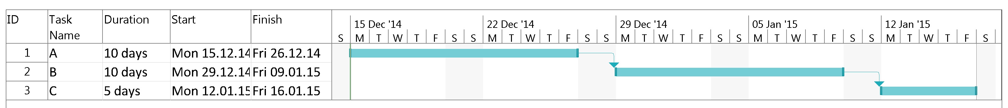
In our example, we have 3 tasks, named “A”, “B” and “C”, and their respective durations is distributed according to the table and the graph below:
| Duration | 0 d | 1 d | 2 d | 3 d | 4 d | 5 d | 6 d | 7 d | 8 d | 9 d | 10 d | 11 d | 12 d | 13 d | 14 d | 15 d | 16 d | 17 d | 18 d | 19 d | 20 d | |
| A | 0% | 0% | 0% | 0% | 0% | 0% | 0% | 0% | 0% | 0% | 0% | 5% | 10% | 25% | 20% | 15% | 10% | 10% | 5% | 0% | 0% | 100% |
| B | 0% | 0% | 0% | 0% | 0% | 0% | 0% | 0% | 0% | 0% | 40% | 30% | 20% | 10% | 0% | 0% | 0% | 0% | 0% | 0% | 0% | 100% |
| C | 0% | 0% | 0% | 0% | 0% | 0% | 50% | 50% | 0% | 0% | 0% | 0% | 0% | 0% | 0% | 0% | 0% | 0% | 0% | 0% | 0% | 100% |
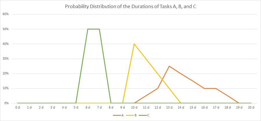
As you can see, there is not a fixed duration for each task as we have that in traditional project management. Rather than that, there are several possible outcomes for each task with respect to the real duration, and the probability of the outcome is distributed as in the graph above. The area below each graph will sum up to 1 (100%) for each task.
If we assume these distributions, how does the probability distribution of sequence of tasks A, B, C look like?
Solution
Level the durations
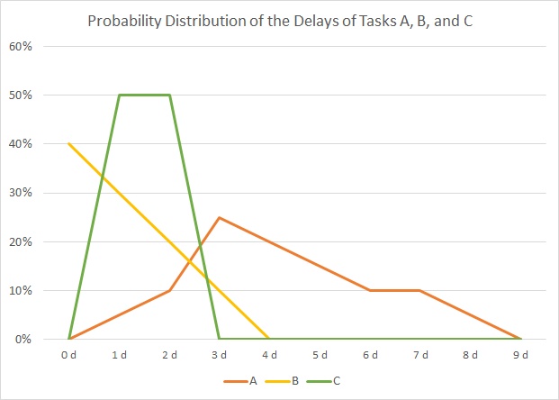
In a first approach, we define a minimum duration for each tasks. This is not mandatory, but it helps us to reduce the memory demand in our algorithm that we will use in a later stage. While we can define any minimum duration from zero to the first non-zero value of the probability distribution, we set them in our example to:
- A: tmin = 10 days
- B: tmin = 10 days
- C: tmin = 5 days (Keep in mind that here, we could also have selected 6 days, for example.)
That approach simply serves to level out tasks with large differences in their minimum duration, it is not necessary for the solution that is described below.
If we do so, then our overall minimum duration is 25 days then which we shall keep in mind right now. We now subtract the minimum duration from each task and get the values in the table and the graph below:
| Delay | 0 d | 1 d | 2 d | 3 d | 4 d | 5 d | 6 d | 7 d | 8 d | 9 d | |
| A | 0% | 5% | 10% | 25% | 20% | 15% | 10% | 10% | 5% | 0% | 100% |
| B | 40% | 30% | 20% | 10% | 0% | 0% | 0% | 0% | 0% | 0% | 100% |
| C | 0% | 50% | 50% | 0% | 0% | 0% | 0% | 0% | 0% | 0% | 100% |
Discrete Convolution
In order to compute the resulting probability distribution, we use the discrete convolution of the probability distributions of tasks A, B, and C, that is: (a∗b∗c). As the discrete convolution is computed as a sum of multiplications, we actually first compute (a∗b) and then convolute the result with c, that is we do ((a∗b)∗c). In order to facilitate our work and enable us to compute sequences of many tasks, we use a C program named faltung.c which processes an input file of probability distributions in a certain format:
- Each description of a probability distribution of a task begins with a statement named # START
- Each description of a probability distribution of a task ends with a statement named # STOP
- Lines with comments must start with a #
- Empty lines are ignored.
- Data lines have an integer value, at least one white space and then a probability. This format can also be used for visualizations with gnuplot.
- The sum of probabilities for each task must add up to 1.00 (= 100%).
- Probability distributions for several tasks can be combined in one input file.
- The output file which the C file faltung.c will generate has the same syntax and can therefore be used as input file for further calculations.
In the example, we use the input:
# START
0 0.00
1 0.05
2 0.10
3 0.25
4 0.20
5 0.15
6 0.10
7 0.10
8 0.05
# STOP
0 0.40
1 0.30
2 0.20
3 0.10
# STOP
0 0.00
1 0.50
2 0.50
# STOP
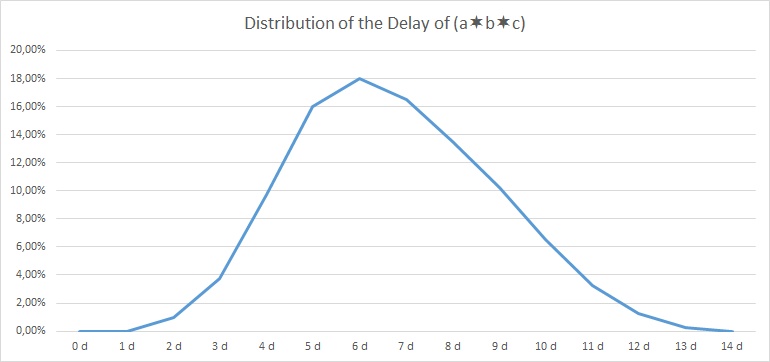
and get the following result:
# The resulting vector is of size: 14
# START
0 0.0000
1 0.0000
2 0.0100
3 0.0375
4 0.0975
5 0.1600
6 0.1800
7 0.1650
8 0.1350
9 0.1025
10 0.0650
11 0.0325
12 0.0125
13 0.0025
# STOP
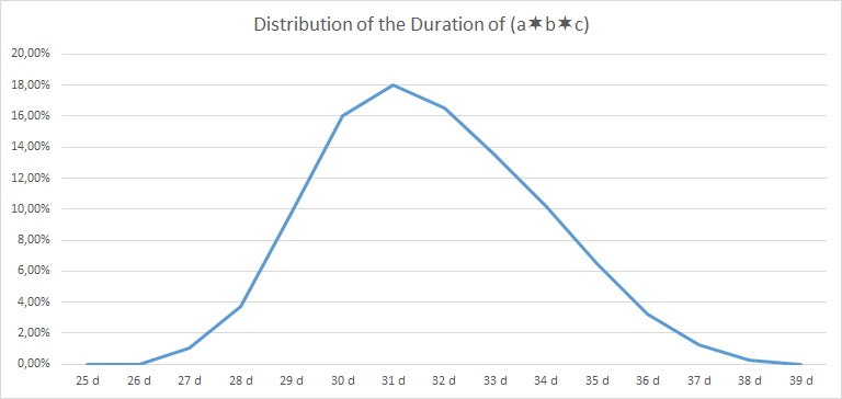
| Delay | 0 d | 1 d | 2 d | 3 d | 4 d | 5 d | 6 d | 7 d | 8 d | 9 d | 10 d | 11 d | 12 d | 13 d | 14 d | |
| (a∗b∗c) | 0,00% | 0,00% | 1,00% | 3,75% | 9,75% | 16,00% | 18,00% | 16,50% | 13,50% | 10,25% | 6,50% | 3,25% | 1,25% | 0,25% | 0,00% | 100% |
Downloads and Hints
- You can download the source code of faltung.c from https://caipirinha.spdns.org/~gabriel/Blog/faltung.c. The source code is in Unix format, hence no CR/LF, but only LF. It can be compiled with gcc -o {target_name} faltung.c. The C program is a demonstration only; no responsibility is assumed for damages resulting from its usage.
- The sample input file is available at https://caipirinha.spdns.org/~gabriel/Blog/input_faltung.dat and can be read with a standard text editor. If is also in Unix format (only LF).
- The maximum delay of the output vector is 99.