Financial Risk and Opportunity Calculation

Financial Risk and Opportunity Calculation

Executive Summary

This blog post offers a method to evaluate n-ary project risks and opportunities from a probabilistic viewpoint. The result of the algorithm that will be discussed, allows to answer questions like:

• What is the probability that the overall damage resulting from incurred risks and opportunities exceeds the value x?
• What is the probability that the overall damage resulting from incurred risks and opportunities exceeds the expected value (computed as ∑(p_i * v_i) for all risks and opportunities)?
• How much management reserve should I assume if the management reserve shall be sufficient with a probability of y%?

The blog post shall also encourage all affected staff to consider more realistic n-ary risks and opportunities rather than the typically used binary risks and opportunities in the corporate world.

This blog post builds on the previous blog post Financial Risk Calculation and improves the algorithm by:

• removing some constraints and errors of the C code
• enabling the code to process risks and opportunities together

Introduction

In the last decades, it has become increasingly popular to not only consider project risks, but also opportunities that may come along with projects. [1] and [2] show aspects of the underlying theory, for example.

In order to accommodate that trend (and also in order to use the algorithm I developed earlier in my professional work), it became necessary to overhaul the algorithm so that it can be used with larger input vectors of risks as well as with opportunities. The current version of the algorithm (faltung4.c) does that.

Examples

Example 1: Typical Risks and Opportunities

In the first example, we will consider some typical risks and opportunities that might occur in a project. The source data for this example is available for download in the file Risks_Opportunities.xlsx.

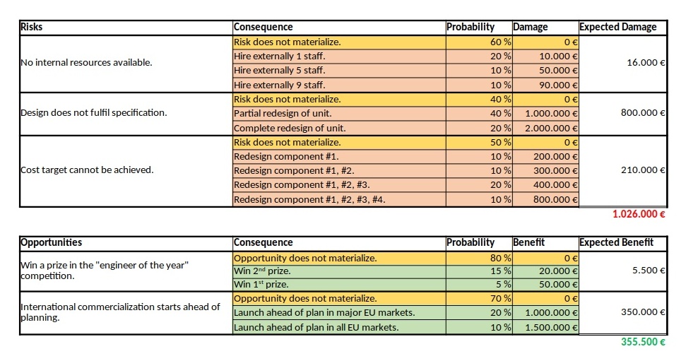
We can see a ternary, a quaternary, and a quinary risk and two ternary opportunities. This is already different from the typical corporate environment in which risks and opportunities are still mostly perceived as binary options (“will not happen” / “will happen”), probably because of a lack of methods to process any other form. At that point I would like to encourage everyone in a corporate environment to take a moment and think whether binary risks only are really still contemporary in the complex business world of today. I believe that they are not.

As already described in the previous blog post Financial Risk Calculation, these values have to copied to a structured format in order to be processed with the convolution algorithm. For the risks and the opportunities shown in the table above, that would turn out to be:

# Distribution of the Monetary Risks and Opportunities
# Risks have positive values indicating the damage values.
# Opportunities have negative values indicating the benefit values.

# START
     0    0.60
 10000    0.20
 50000    0.10
 90000    0.10
# STOP

# START
       0  0.40
 1000000  0.40
 2000000  0.20
# STOP

# START
      0   0.50
 200000   0.10
 300000   0.10
 400000   0.20
 800000   0.10
# STOP

# START
       0   0.80
  -20000   0.15
  -50000   0.05
# STOP

# START
       0   0.70
-1000000   0.20
-1500000   0.10
# STOP

Note that risks do have positive (damage) values whereas opportunities have negative (benefit) values. That is inherently programmed into the algorithm, but of course, could be changed in the C code (for those who like it the opposite way).
After processing the input with:

cat risks_opportunities_input.dat | ./faltung4.exe > risks_opportunities_output.dat

the result is stored in the file risks_opportunities_output.dat which is lengthy and therefore not shown in full here on this page. However, let’s discuss about some important result values at the edge of the spectrum:

# Convolution Batch Processing Utility (only for demonstration purposes)
# The resulting probability density vector is of size: 292
# START
  -1550000   0.0006000000506639
...
   2890000   0.0011200000476837
# STOP

# The probability values are:
  -1550000   0.0006000000506639
  -1540000   0.0008000000625849
...
         0   0.2721000205919151
...
   2870000   0.9988800632822523
   2890000   1.0000000633299360

The most negative outcome corresponds to the possibility that no risk occurs, but that all opportunities realize with their best value. In our case this value is 1,550,000 €, and from the corresponding line in the density vector we see that the probability of this occurring is only 0.06%.
The most positive outcome corresponds to the possibility that no opportunity occurs and that all risks realize with their worst value. On our case, this is 2,890,000 €, and the probability of this to occur is 0.11%. In between those extreme values, there are 290 more possible outcomes (292 in total) for a benefit or damage.
Note that the probability density vector is enclosed in the tags #START and #STOP so that it can directly be used as input for another run of the algorithm.

The second part of the output contains the probability vector which (of course) also has 292 in this example. The probability vector is the integration of the probability density vector and sums up all probabilities. The first possible outcome (most negative value) therefore starts with the same probability value, but the last possible outcome (most positive value) has the probability 1. In our case, the probability is slightly higher as 1, and this is due to the fact that float or double variables in C do not have infinite resolution. In fact, already when converting a number with decimals to a float or double value, you most probably encounter imprecisions (unless the value is a multiple or fraction of 2).

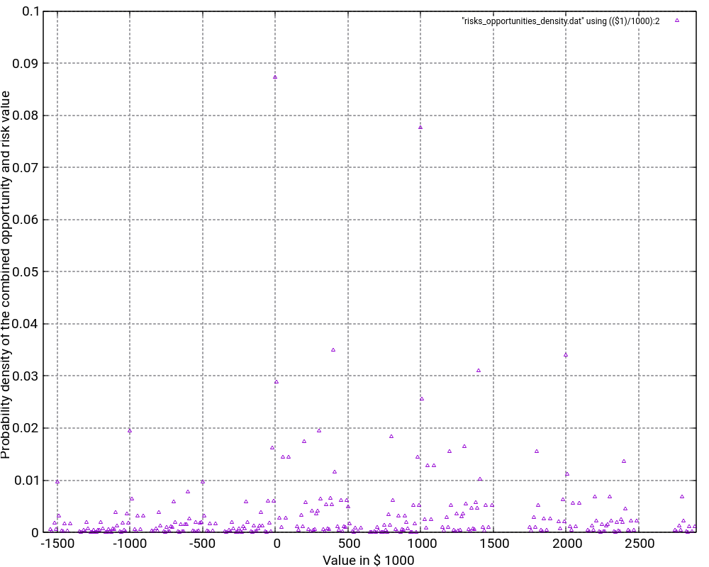
The file Risks_Opportunities.xlsx contains the input vector and the output of the convolution as well as some graphic visualizations in Excel. However, for large output values, I do not recommend to process or visualize them in Excel, but instead, I recommend to use gnuplot for the visualization. The images below show the probability density distribution as well as (1 – probability distribution) as graphs generated with gnuplot.

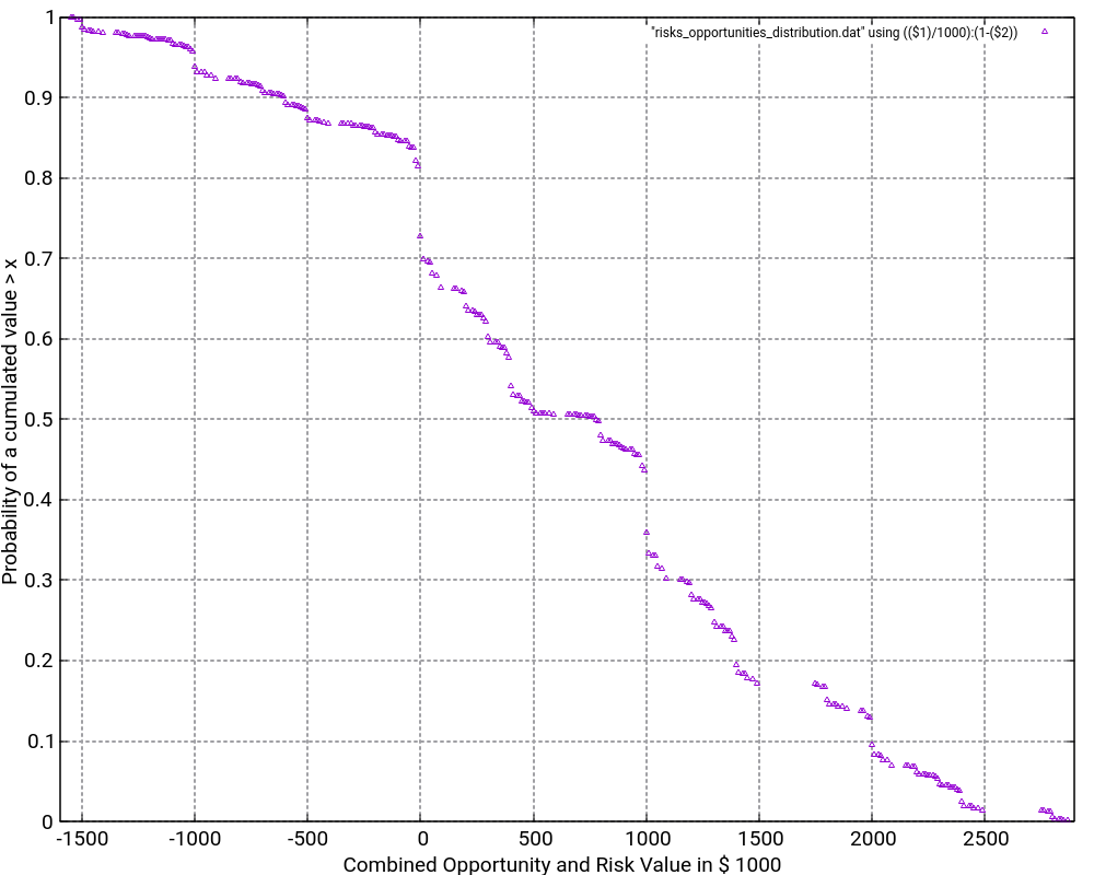
What is the purpose of the (1 – Probability distribution) graph? The purpose is to answer the question: “What is the probability that the damage value is higher as x?”
Let’s look what the probability of a damage value of more than 1,000,000 € is? In order to do so, we locate “1000” on the x-axis and go vertically up until we reach the graph. Then, we branch to the left and read the corresponding value on the y-axis. In our case, that would be something like 36%. This means that there is a probability of 36% that thus project experiences a damage of more than 1,000,000 €. This is quite a notable risk, something which one would probably not guess by just looking at the expected damage value of 1,026,000 € listed in the Excel table.
And even damage values of more than 2,000,000 € can still occur with some 10% of probability.
The graph would always start relatively on the top left and finish on the bottom right. Note that the graph does not start at 1.0 because there is a small chance that the most negative value (no risks, but the maximum of the opportunities realized) happens. However, the graph reaches the x-axis at the most positive value. Therefore, it is important asking the question “What is the probability that the damage value is higher than x?” rather than asking the question “What is the probability that the damage value is than x or higher?” The second question is incorrect although the difference might be minimal when many risks and opportunities are used as input.

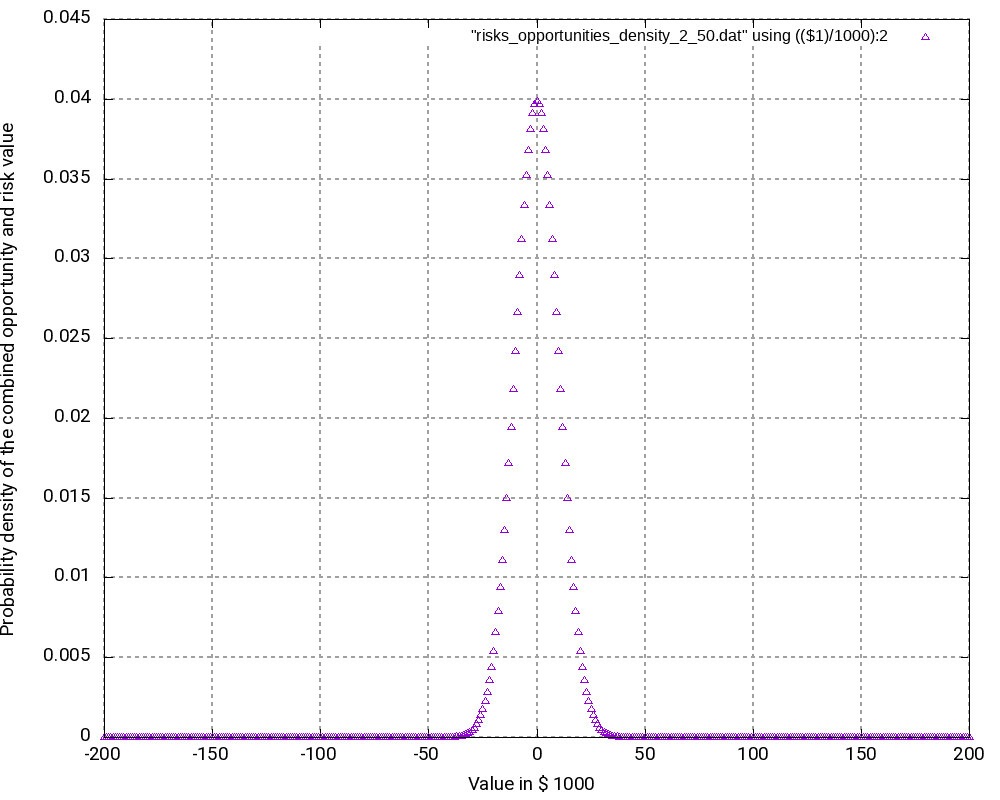
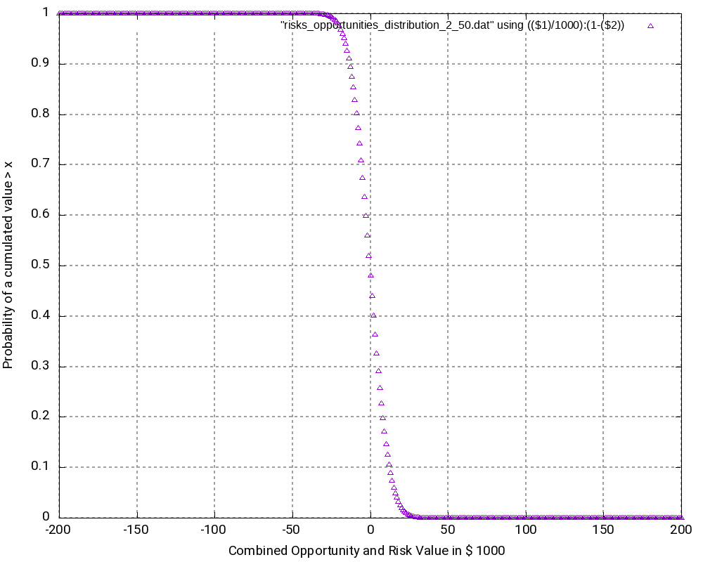
Example 2: Many binary risks and opportunities of the same value

This example is not a real one, but it shall help us to understand the theory behind the algorithm. In this example, we have 200 binary risks and 200 binary opportunities with a damage or benefit value of 1,000 € and a probability of occurrence of 50%.

# Risks have positive values indicating the damage values.
# Opportunities have negative values indicating the benefit values.

# START
    0   0.50
 1000   0.50
# STOP

# START
    0   0.50
-1000   0.50
# STOP
...

From this, we can already conclude that the outcomes are in the range [-200,000 €; +200,000 €] corresponding to the rare events “no risk materializes, but all opportunities materialize” respectively “no opportunity materializes, but all risks materialize”. As the example is simple in nature, we can also conclude immediately that the possibility of such an extreme outcome is

p = 0.5^(200+200) = 3.87259*10^-121

and that is really a very low probability. We might also guess that the outcome value zero would have a relatively high probability as we can expect this value to be reached by many different combinations of risks and opportunities.

When we look at the resulting probability density curve and the resulting probability distribution, we can see a bell-shaped curve in the probability density and the resulting S curve as the integration of the bell-shaped curve. While the curve resembles a Gaussian distribution, this is not the case in reality as our possible outcomes are bound by a lower negative value and an upper positive value whereas a strict Gaussian distribution has a probability (and be it minimal only) for any value on the x-axis.

Let us have a closer look at some values in the output tables:

# Convolution Batch Processing Utility (only for demonstration purposes)
# The resulting probability density vector is of size: 401
# START
   -200000   0.0000000000000000
   -199000   0.0000000000000000
...
     -2000   0.0390817747440756
     -1000   0.0396709472276547
         0   0.0398693019637929
      1000   0.0396709472276547
      2000   0.0390817747440756
...
    199000   0.0000000000000000
    200000   0.0000000000000000
# STOP

# The probability values are:
   -200000   0.0000000000000000
   -199000   0.0000000000000000
...
     -2000   0.4403944017904490
     -1000   0.4800653490181037
         0   0.5199346509818966
      1000   0.5596055982095512
      2000   0.5986873729536268
...
    199000   0.9999999999999996
    200000   0.9999999999999996

The following observations can be made:

• The most negative outcome (-200,000 €) and the most positive outcome (+200,000 €) can only be reached in one constellation and have, as calculated above, minimal probability of occurrence. Therefore, the probability density vector shows all zero in the probability.
• The outcome 0 has the highest probability of all possible outcomes (3.99%), and outcomes close to 0 have a similarly high probability. Hence, it is very probable that the overall outcome of a project with this (artificially constructed) risk and opportunity pattern is around 0.
• It may astonish at first that in the probability distribution (not the probability density), the value 0 is attributed to a probability of 51.99% rather than to 50.00%. However, we must keep in mind that the values in the probability distribution answer the question: “What is the probability that the outcome is > x?” and not “… ≥ x?” That makes the difference.
• At the upper end of the probability distribution (+200,000 €), we would expect the probability to be 1.0 rather than a value below that. However, here, the limited resolution of even double variables in C result in the fact that errors in the precision of arithmetic results add up. This might be improved by using long double as probability variable.

Example 3

The third example is similar to the second one, but it only contains risks, that is, we leave away all opportunities from the second example. Consequently, outcomes (damages) lie in the interval [0; +200,000 €]. The outcomes at the edges of the interval have the lowest probability of occurrence, in this case:

p = 0.5²⁰⁰ = 6.22302*10^-61

While this probability of occurrence is much higher than the one for the edge values in Example 2, it is still very low.

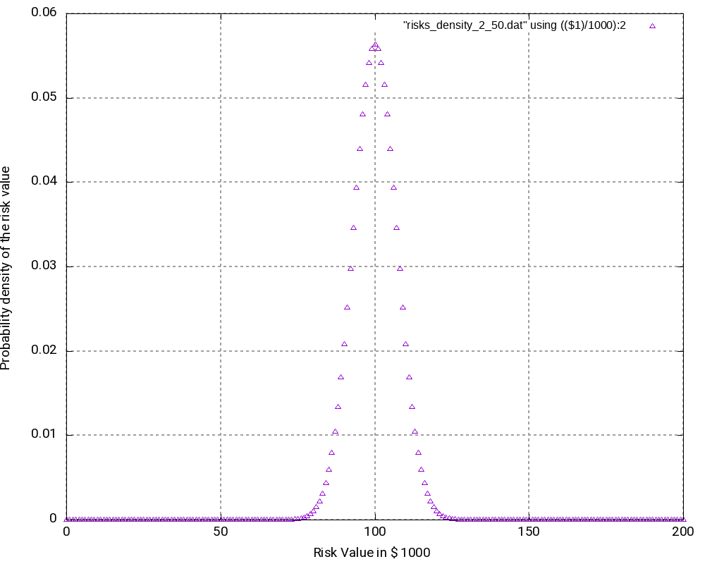
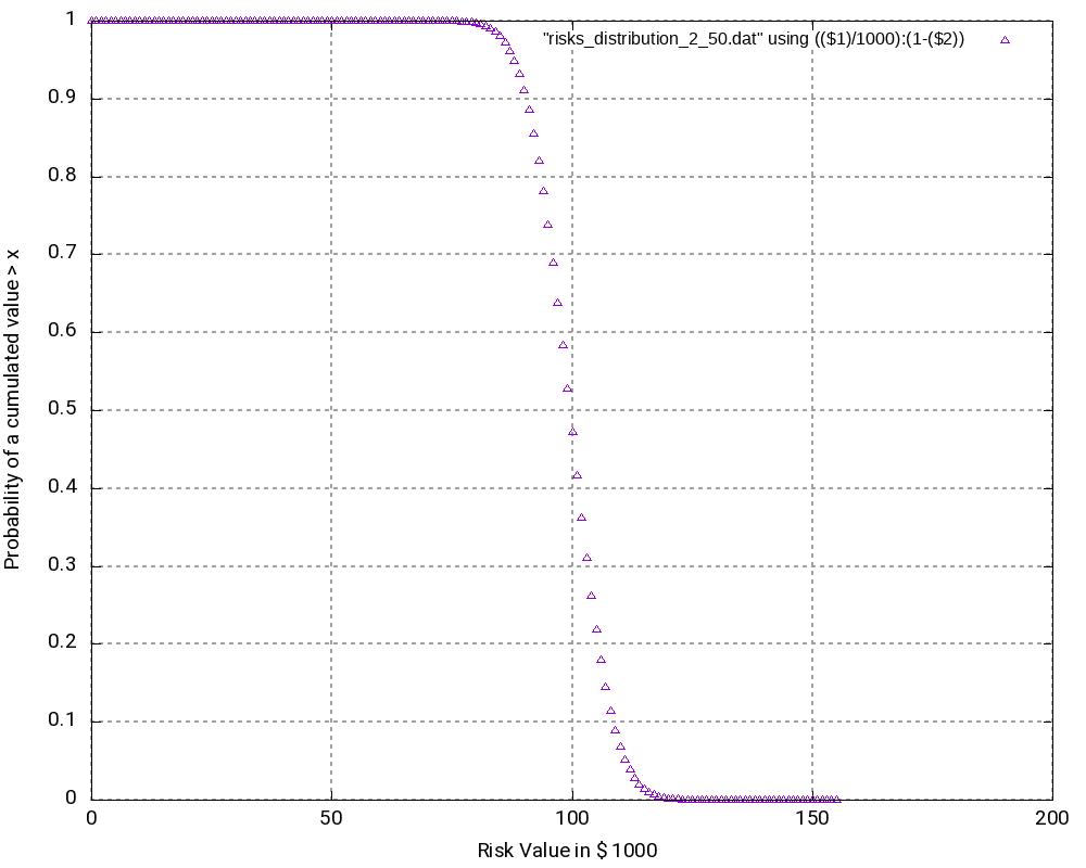
As we can see (and this could be expected somewhat), the most probably outcome now is a damage of +100,000 €, again the value in the middle of the interval which now has a probability of occurrence of 5.63% (higher than in the second example). While the curves in the second and in the third example look very similar, the curves are “steeper” in the third example.

# Convolution Batch Processing Utility (only for demonstration purposes)
# The resulting probability density vector is of size: 201
# START
         0   0.0000000000000000
      1000   0.0000000000000000
...
     99000   0.0557905732764915
    100000   0.0563484790092564
    101000   0.0557905732764915
...
    199000   0.0000000000000000
    200000   0.0000000000000000
# STOP

# The probability values are:
         0   0.0000000000000000
      1000   0.0000000000000000
...
     99000   0.4718257604953718
    100000   0.5281742395046283
    101000   0.5839648127811198
...
    199000   1.0000000000000002
    200000   1.0000000000000002

Conclusion

This blog post shows that with the help of the algorithm faltung4.c, it has become possible to computer probability densities and probability distributions of combined risks and opportunities and answer valid and important questions with respect to the project risk and the monetary reserves (aka “management reserve”) that should be attributed to a project with a certain portfolio of risks and opportunities.

Outlook

The algorithm may be enlarged so that it can accommodate start and finish dates of risks and opportunities. In this case, probability densities and probability distributions can be computed for any point in time that changes the portfolio of risks and opportunities due to the start or finish of a risk or opportunity. In this case, the graphs will become 3-dimensional and look somewhat like a “mountain area”. This would have relevance in the sense that some projects might start heavily on the risky side and opportunities might only become available later. For such projects, there is a real chance that materialized risks result in a large cash outflow which later is then partially compensated by materialized opportunities.

Sources

• [1] = Balancing project risks and opportunities
• [2] = Project opportunity – risk sink or risk source?

Files

• Risks_Opportunities.xlsx contains the example table as well as the result tables of the analysis, graphs and some scripting commands.
• faltung4.c contains the C program code that was used for the analysis.
• Example 1:
  • risks_opportunities_input.dat is the input table.
  • risks_opportunities_output.dat is the output table which contains the probability density and the probability distribution.
  • risks_opportunities_density.dat is the output table containing the probability density only.
  • risks_opportunities_density.png is a graphic visualization of the probability density with gnuplot.
  • risks_opportunities_distribution.dat is the output table containing the probability distribution only.
  • risks_opportunities_distribution.png is a graphic visualization of (1 – probability distribution) with gnuplot.
• Example 2:
  • risks_opportunities_input_2_50.dat is the input table.
  • risks_opportunities_output_2_50.dat is the output table which contains the probability density and the probability distribution.
  • risks_opportunities_density_2_50.dat is the output table containing the probability density only.
  • risks_opportunities_density_2_50.png is a graphic visualization of the probability density with gnuplot.
  • risks_opportunities_distribution_2_50.dat is the output table containing the probability distribution only.
  • risks_opportunities_distribution_2_50.png is a graphic visualization of (1 – probability distribution) with gnuplot.
• Example 3:
  • risks_input_2_50.dat is the input table.
  • risks_output_2_50.dat is the output table which contains the probability density and the probability distribution.
  • risks_density_2_50.dat is the output table containing the probability density only.
  • risks_density_2_50.png is a graphic visualization of the probability density with gnuplot.
  • risks_distribution_2_50.dat is the output table containing the probability distribution only.
  • risks_distribution_2_50.png is a graphic visualization of (1 – probability distribution) with gnuplot.

Usage

Scripts and sequences indicating how to use the algorithm faltung4.c can be found in the table Risks_Opportunities.xlsx on the tab Commands and Scripts. Please follow these important points:

• The input file which represents n-ary risks and n-ary opportunities as well as their probabilities of occurrence, has to follow a certain structure which is hard-coded in the algorithm faltung4.c. A risk or opportunity is always enclosed in the tags # START and # STOP.
• Lines starting with “#” are ignored as are empty lines.
• The probabilities of occurrence of an n-ary risk or an n-ary opportunity must sum up to 1.0.
• The C code can be compiled with a standard C compiler, e.g., gcc, with the sequence:

gcc -o faltung4.exe faltung4.c

• The input file is computed and transformed into an output file with the sequence:

cat input_file.dat | ./faltung4.exe > output_file.dat

• The output file consists of two parts:
  • a resulting probability density which has the same structure as the input file (with the tags # START and # STOP)
  • a resulting probability distribution
• In order to post-process the output, e.g., with gnuplot, you can help yourself with standard Unix tools like head, tail, wc, cat, etc.
• The output file is structured in a way so that it can be easily used for visualizations with gnuplot.

Disclaimer

• The program code and the examples are for demonstration purposes only.
• The program shall not be used in production environments.
• While the program code has been tested, it might still contain errors.
• Due to rounding errors with float variables, you might experience errors depending on your input probability values when reading the input vector.
• The program code has not been optimized for speed.
• The program code has not been written with cybersecurity aspects in mind.
• This method of risk and opportunity assessment does not consider that risks and opportunities in projects might have different life times during the project, but assumes a view “over the whole project”. In the extreme case, for example, that risks are centered at the beginning and opportunities are centered versus the end of a project, it might well be possible that the expected damage/benefit of the overall project is significantly exceeded or significantly subceeded.