Author: Gabriel Rüeck
Getting around Corporate VPN Restrictions
Executive Summary
This blog post explains how Policy Routing on a Linux server in the Home Office can help you to bypass access restrictions by a corporate VPN to your local LAN.
Background
The need for this approach surged when I realized that while being in the corporate VPN with my company notebook, I could not access my home network anymore.
Preconditions
In order to use the approach described here, you should:
- … have access to a Linux machine which is already properly configured on its principal network interface (e.g., eth0) and which has an additional network card (e.g., eth1) available
- … have knowledge of routing concepts, networks, some understanding of shell scripts and configuration files
- … have already setup meaningful services like NTP, samba or MariaDB / MySQL on the Linux machine
- … know related system commands like sysctl
- … familiarize yourself with [1] and read at least a bit through [2]
Description and Usage
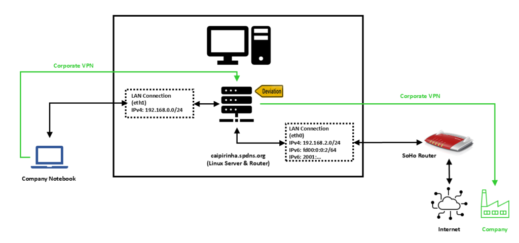
In this setup, we have a full-blown SoHo Linux server on an internal network 192.168.2.0/24 that is also used by all other devices in the same home. For the approach described here, this Linux server needs to be equipped with an additional network card (eth1), and we will use this connection exclusively in order to connect the company notebook. A DHCP and DNS server on the Linux server shall span the network 192.168.0.0/24 on the interface eth1, and the company notebook will get an IP address in this network. We assume that for remote work (Home Office), the user has to use a corporate VPN which is then channeled through our Linux server. For the approach described here, it is important that the corporate VPN on the company notebook does not channel all traffic of the company notebook through the VPN, but that it is a split VPN that leaves some routes outside of the VPN. Many corporate VPN are essentially split VPN and typically exclude IP ranges that connect to Microsoft® services (M365, Teams, SharePoint, etc.) or dedicated streaming services used by the company so that this traffic is not led through the company (it would anyway be fed into the company and directly be sent out to Microsoft® only using precious bandwidth of the company’s internet connection). We will single out one IP address of the IP ranges that are outside the corporate VPN and use the fact that legitimate traffic which might go to this IP address almost certainly will be either on port 80 (http) or on port 443 (https). An iptables command will help us to deviate traffic on this one IP address that shall go to dedicated services on our Linux server.
We need some auxiliary services in order to make things work perfectly, and they are described in the following sections.
Setting up eth1
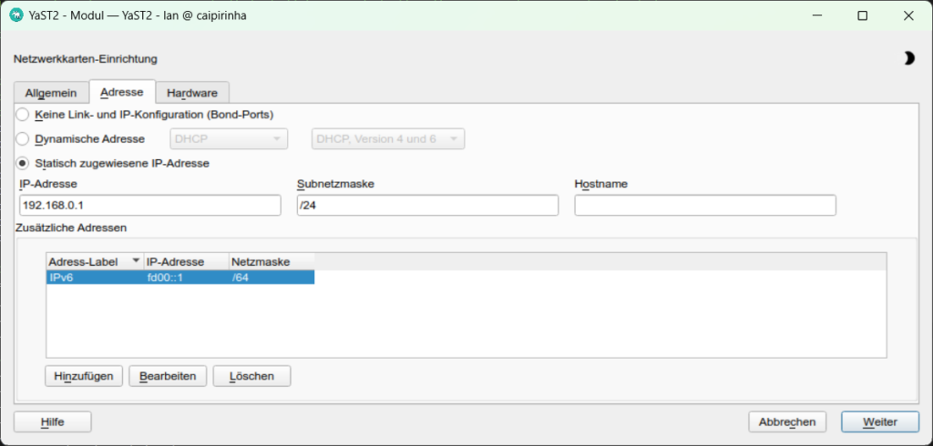
The first step is to set up the interface eth1 and to assign static IP addresses for IPv4 and IPv6. In order to make life easy for me, I use YaST2 on my openSuSE system and assign the addresses 192.168.0.1 and fd00::1 to the Linux server on eth1.
Providing DHCP and DNS on eth1
The company notebook needs to get an IP address when it is booted up, and since it is connected only to eth1 on the Linux server, this means that the Linux server shall provide an IP address via DHCP so that we do not have to configure a static IP on the company notebook. The package dnsmasq can provide both DHCP as well as cache DNS. That is very practical as it allows us for example, to have only DNS on eth0 where the SoHo router already is the DHCP master, but to configure both DHCP and a caching DNS on eth1. The following configuration file will exactly do that (it uses only a subset of the capabilities of dnsmasq):
/etc/dnsmasq.conf
# Never forward addresses in the non-routed address spaces.
bogus-priv

# If you don't want dnsmasq to read /etc/resolv.conf or any other
# file, getting its servers from this file instead (see below), then
# uncomment this.
no-resolv

# If you don't want dnsmasq to poll /etc/resolv.conf or other resolv
# files for changes and re-read them then uncomment this.
no-poll

# Add other name servers here, with domain specs if they are for
# non-public domains.
server=8.8.8.8
server=8.8.4.4
server=9.9.9.9
server=1.1.1.1

# If you want dnsmasq to listen for DHCP and DNS requests only on
# specified interfaces (and the loopback) give the name of the
# interface (eg eth0) here.
# Repeat the line for more than one interface.
interface=eth0
interface=eth1

# If you want dnsmasq to provide only DNS service on an interface,
# configure it as shown above, and then use the following line to
# disable DHCP and TFTP on it.
no-dhcp-interface=eth0

# Uncomment this to enable the integrated DHCP server, you need
# to supply the range of addresses available for lease and optionally
# a lease time. If you have more than one network, you will need to
# repeat this for each network on which you want to supply DHCP
# service.
dhcp-range=tag:eth1,192.168.0.10,192.168.0.254,24h

# Enable DHCPv6. Note that the prefix-length does not need to be specified
# and defaults to 64 if missing/
dhcp-range=tag:eth1,fd00:0:0:0::A, fd00:0:0:0::C8, 64, 24h

# Assign a pseudo-static IPv4 to the the company notebook identified by its MAC.
# Assign a pseudo-static IPv6 to the the company notebook identified by its DUID.
# Note the MAC addresses CANNOT be used to identify DHCPv6 clients.
dhcp-host=80:3f:5d:d2:4b:57,FHD4QV3,192.168.0.195,24h
dhcp-host=id:00:01:00:01:2c:e6:bc:51:ac:91:a1:61:03:30,FHD4QV3,[fd00::c3/64]

# Set the NTP time server addresses
dhcp-option=option:ntp-server,192.168.2.3

# Send Microsoft-specific option to tell windows to release the DHCP lease
# when it shuts down. Note the "i" flag, to tell dnsmasq to send the
# value as a four-byte integer - that's what Microsoft wants. See
# https://learn.microsoft.com/en-us/openspecs/windows_protocols/ms-dhcpe/4cde5ceb-4fc1-4f9a-82e9-13f6b38d930c
dhcp-option=vendor:MSFT,2,1i

# Include all files in a directory which end in .conf
conf-dir=/etc/dnsmasq.d/,*.conf
In this configuration, we can see that on eth0, we will not enable DHCP (Option no-dhcp-interface=eth0). On eth1, we want DHCP to be active. Furthermore, we propagate the server’s address 192.168.2.3 as NTP server. For this, the NTP service needs to be enabled, of course, otherwise that would be pointless.
With the configuration option dhcp-host, we can assign a pseudo-static IPv4 address (192.168.0.195) to the company notebook identified by its MAC address. And using the same option for a second time, we can also assign a pseudo-static IPv6 address to the company notebook. However, in order to accomplish this, we need to know the DHCP Unique Identifier (DUID) of the company notebook. With dnsmasq, we can obtain the DUID by leaving out the option dhcp-host at first and then scanning in the log file of dnsmasq (or, in the syslog if no dedicated log file has been specified) which DUID the notebook has. In the log file, we might find entries like:
2026-02-27T09:51:39.478262+01:00 caipirinha dnsmasq-dhcp[14776]: DHCPSOLICIT(eth1) 00:01:00:01:2c:e6:bc:51:ac:91:a1:61:03:30
2026-02-27T09:51:39.478460+01:00 caipirinha dnsmasq-dhcp[14776]: DHCPADVERTISE(eth1) fd00::c3 00:01:00:01:2c:e6:bc:51:ac:91:a1:61:03:30 fhd4qv3
The DUID can then be identified as 00:01:00:01:2c:e6:bc:51:ac:91:a1:61:03:30.
dnsmasq uses the file /etc/hosts as well as upstream DNS servers for its own DNS service. The advantage of this is that – if your file /etc/hosts is properly maintained – you can also use the device names listed there. As upstream DNS servers from which dnsmasq itself gets the IP resolution, I have configured four popular ones (8.8.8.8, 8.8.4.4, 9.9.9.9, 1.1.1.1), but you could also just list the IP of your SoHo router or of the DNS resolver of your internet provider.
Providing web proxy services
If we want to use unrestricted and unfiltered internet also on the company notebook, then we need to set up a web proxy on our Linux server and use a separate browser on the company notebook on which we configure the Linux server as web proxy. As on company notebooks, you might not be allowed to install software by yourself, Mozilla Firefox, Portable Edition might be an option. This is a browser that does not require installation but can just be placed on the hard disk of the company notebook. In this browser, you can configure a dedicated proxy server without having to change the system configuration or default proxy setting of the company notebook. On the Linux server, the package tinyproxy is an easy-to-configure and lightweight proxy server well suited for our purpose. Below is a typical configuration of tinyproxy. The configuration option Port sets the port on which tinyproxy will listed for incoming connections, in our case I chose 4077.
/etc/tinyproxy.conf
# User/Group: This allows you to set the user and group that will be
# used for tinyproxy after the initial binding to the port has been done
# as the root user. Either the user or group name or the UID or GID
# number may be used.
#
User tinyproxy
Group tinyproxy

# Port: Specify the port which tinyproxy will listen on.  Please note
# that should you choose to run on a port lower than 1024 you will need
# to start tinyproxy using root.
#
Port 4077

# Bind: This allows you to specify which interface will be used for
# outgoing connections.  This is useful for multi-home'd machines where
# you want all traffic to appear outgoing from one particular interface.
#
Bind 192.168.2.3

# Timeout: The maximum number of seconds of inactivity a connection is
# allowed to have before it is closed by tinyproxy.
#
Timeout 600

# LogFile
#
LogFile "/var/log/tinyproxy/tinyproxy.log"

# LogLevel: Warning
#
# Set the logging level. Allowed settings are:
#	Critical	(least verbose)
#	Error
#	Warning
#	Notice
#	Connect		(to log connections without Info's noise)
#	Info		(most verbose)
#
LogLevel Warning

# PidFile
#
PidFile "/var/run/tinyproxy/tinyproxy.pid"

# XTinyproxy: Tell Tinyproxy to include the X-Tinyproxy header, which
# contains the client's IP address.
#
XTinyproxy Yes

# MaxClients: This is the absolute highest number of threads which will
# be created. In other words, only MaxClients number of clients can be
# connected at the same time.
#
MaxClients 400

# Allow: Customization of authorization controls. If there are any
# access control keywords then the default action is to DENY. Otherwise,
# the default action is ALLOW.
#
Allow 127.0.0.1
Allow ::1
Allow 192.168.0.0/16

# ViaProxyName: The "Via" header is required by the HTTP RFC, but using
# the real host name is a security concern.  If the following directive
# is enabled, the string supplied will be used as the host name in the
# Via header; otherwise, the server's host name will be used.
#
ViaProxyName "tinyproxy"

# Filter: This allows you to specify the location of the filter file.
#
Filter "/etc/tinyproxy/filter"

# FilterURLs: Filter based on URLs rather than domains.
#
FilterURLs On

# FilterDefaultDeny: Change the default policy of the filtering system.
# If this directive is commented out, or is set to "No" then the default
# policy is to allow everything which is not specifically denied by the
# filter file.
#
# However, by setting this directive to "Yes" the default policy becomes
# to deny everything which is _not_ specifically allowed by the filter
# file.
#
FilterDefaultDeny No
tinyproxy also allows filtering of internet domains. I know I said before that we want unrestricted and unfiltered internet access, but in this case, we can use the file /etc/tinyproxy/filter in order to filter out nasty and annoying advertisement and tracking domains. Suitable filter lists can be found on the internet and can just be copied to /etc/tinyproxy/filter. Or you might add just these domains whose advertisements annoy you most when you access web pages. I personally use a mixture of both.
Re-routing traffic to our server
In my personal case, the corporate VPN client (a Cisco VPN client) is so helpful that it provides me with the IP ranges that are excluded from the corporate VPN. Out of these IP ranges, I did pick one IP address, in my case, 192.229.232.200. The selection was completely arbitrary; I could have chosen any other IP address from the IP ranges that are excluded from the corporate VPN. The following commands prepare the Linux server for our desired setup:
ip link set eth1 up
iptables -t nat -A POSTROUTING -s 192.168.0.0/24 -o eth0 -j SNAT --to-source 192.168.0.1
ip6tables -t nat -A POSTROUTING -s fd00:0:0:0::/64 -o eth0 -j MASQUERADE
iptables -t nat -A PREROUTING -i eth1 -p tcp -d 192.229.232.200 --match multiport --dports 22,445,3306,4077 -j DNAT --to 192.168.2.3
systemctl start dnsmasq.service
systemctl start tinyproxy.service
Let us discuss these commands in detail:
- The first command brings up the network interface eth1. This command might not be necessary if you have a switch connected to eth1 of the Linux Server or if the company notebook is powered up before you boot up the Linux server. Otherwise, if you boot up the Linux server and nothing is connected to eth1, the interface might not come up.
- The second command translates traffic from the network on eth1 to the SoHo network 192.168.2.0/24 and to the Linux server’s address on that network (192.168.2.3). Of course, IPv4 routing needs to be enabled on the Linux server. This command enables that (even without the corporate VPN active), the company notebook can get access to the internet from its otherwise isolated network 192.168.0.0/24.
- The third command does the same for the IPv6 domain and the network fd00:0:0:0::/64 on eth1. Probably we would not even need IPv6 on the network of the company notebook, few companies already work with IPv6. If we leave IPv6 away, we should however also delete the configuration option dhcp-host for IPv6 in /etc/dnsmasq.conf.
- The fourth command is very important. It tells the server to deviate connections on one of the TCP ports 22, 445, 3306, 4077 originally destined to the IP address 192.229.232.200 to the new IP address 192.168.0.1, the IP address of the Linux server on eth1.
- The fifth and sixth command start the services dnsmasq and tinyproxy.
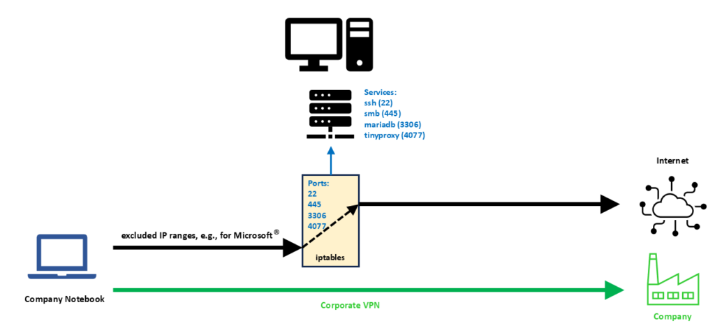
We can see from the fourth command that the scope for deviating connections to the Linux server is very narrow. First, we only consider TCP connections, and we single out only four IP ports that probably otherwise would not be used in conjunction with the IP address 192.229.232.200. With this, we can access the following services on our Linux server:
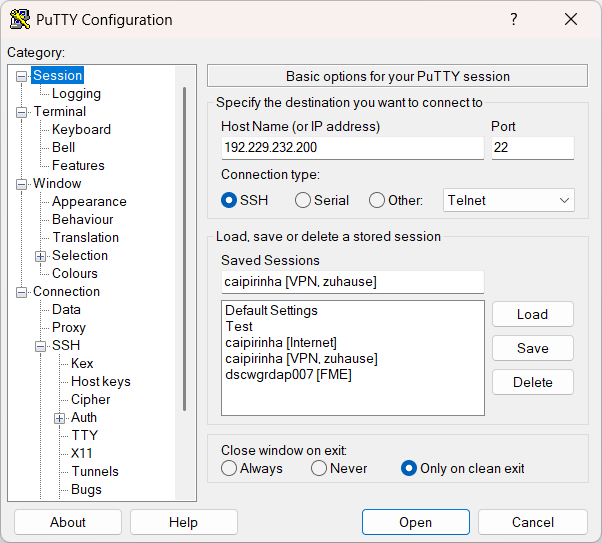
- ssh (Port 22): On the company notebook, we have to configure our ssh client (e.g., puTTY) for a connection to 192.229.232.200:22.
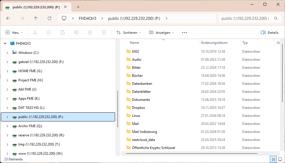
- smb (Port 445): Of course, the Linux server must have a smb service running already; the configuration of it is not part of this article. Then, on the company notebook, we can access a network drive by using \\192.229.232.200\network_share.
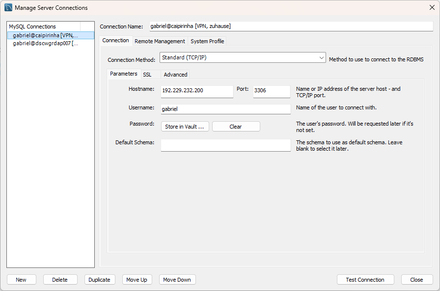
- mariadb / mysql (Port 3306): Of course, the Linux server must have a mysql service running already; the configuration of it is not part of this article. Then, on the company notebook, we can access the service for example with the MySQL Workbench by connecting to 192.229.232.200:3306.
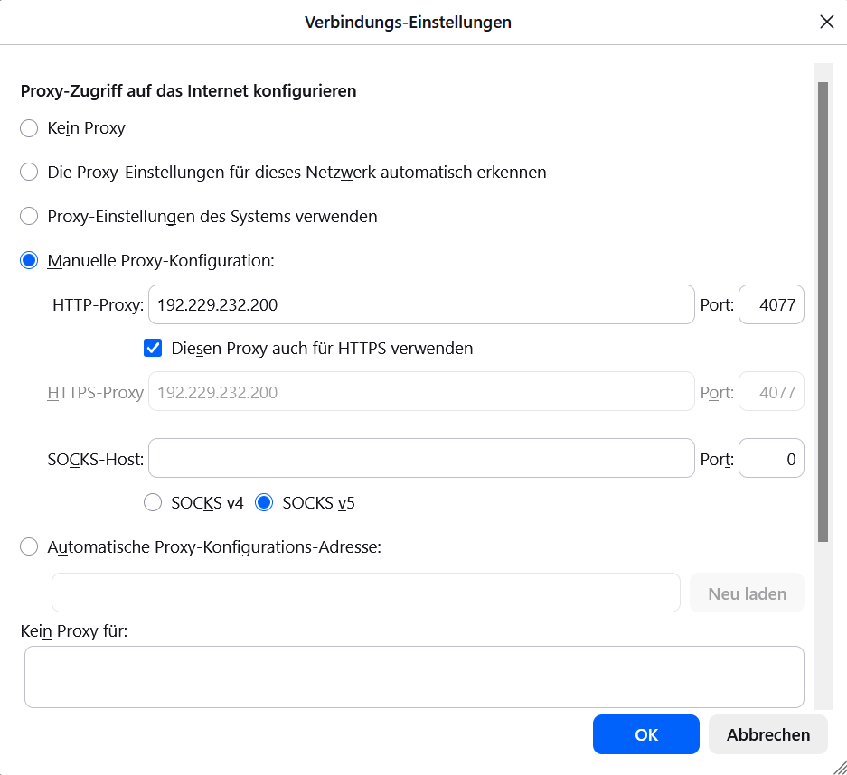
- tinyproxy (Port 4077): We configure Mozilla Firefox, Portable Edition and set the proxy to 192.229.232.200, Port 4077 for both http and https.
The following images show the configuration of related programs and apps on the company notebook.
Of course, you can modify the iptables command (fourth command above) to deviate even more ports, depending on the services that you have available on your own Linux server.
Conclusion
With a second LAN, DHCP, DNS, a proxy server like tinyproxy, some clever commands and a split corporate VPN, we can bypass corporate VPN restrictions that would not allow us to access our local network and services on our Linux server otherwise. With an additional browser on the company notebook like Mozilla Firefox, Portable Edition, this will even enable us to bypass restrictions and browsing policies that corporations might have put forward.
Having said that, I would always recommend you stick to the IT regulations of your company, of course…
Sources
Getting around TV App Geo-Blocking
Executive Summary
This blog post explains how Policy Routing on a Linux server together with commercial VPNs to other countries can help you to put your client devices (TV, smartphones) logically into the internet of other countries in order to get around geo-blocking.
Background
The idea or merely, the need for this approach, surged when I installed an app of a Portuguese TV provider and could not even watch the news journal due to geo-blocking. Additionally, I wanted to have a comfortable solution with which I can switch the TV to different countries while I am sitting in my TV chair with my smartphone at hand 😁.
Preconditions
In order to use the approach described here, you should:
- … have access to a Linux machine which is already properly configured on its principal network interface (e.g., eth0)
- … have the package openvpn installed on the Linux machine (preferably from a repository of your Linux distribution)
- … have access to a commercial VPN provider allowing you to run several parallel client connections on the same machine
- … have knowledge of routing concepts, networks, some understanding of shell scripts and configuration files
- … know related system commands like sysctl
- … familiarize yourself with [1], [3], [4], [5]
Description and Usage
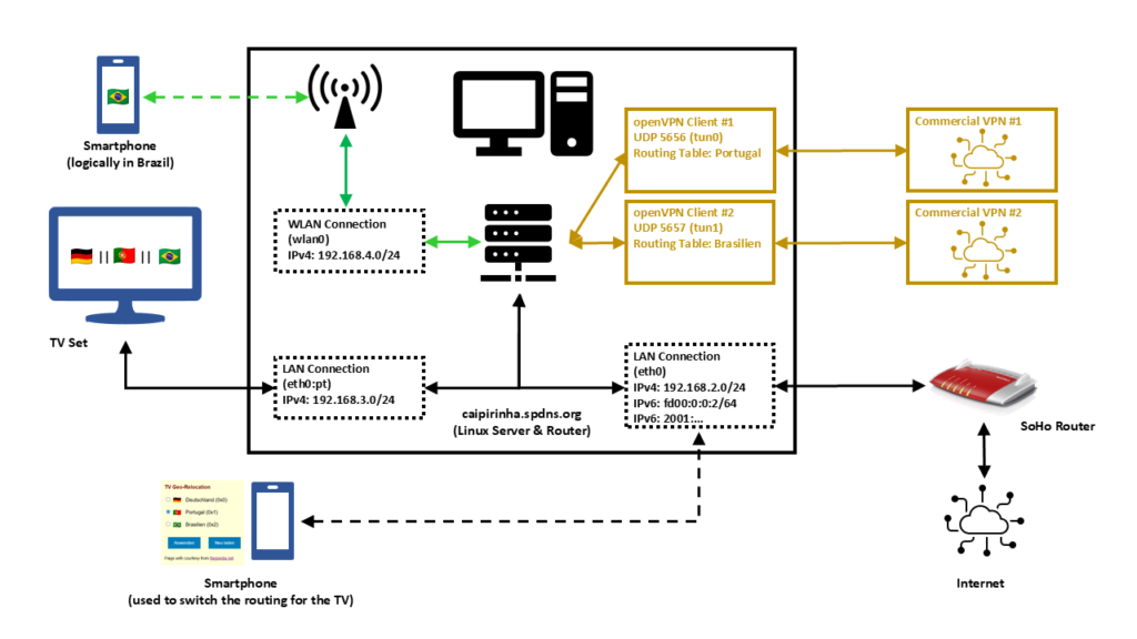
In this setup, we have a full-blown SoHo Linux server on an internal network 192.168.2.0/24 that is also used by all other devices in the same home. Subsequently, we will connect this Linux server via a commercial VPN to two endpoints, one endpoint in Portugal and one endpoint in Brazil. We will also create two additional networks for our SoHo environment:
- 192.168.4.0/24 will be spread via WLAN (WiFi) and will constantly logically be “in Brazil”. This network can simply be selected by a smartphone at home, and the smartphone will have a Brazilian internet connection while still being able to access all resources in the home network.
- 192.168.3.0/24 will an overlay on our wired SoHo network. The TV set will be the only client in this network. We will make the endpoint of this network selectable, that is, one shall be able to select whether this network is in Germany, in Portugal, or in Brazil.
That setup is suited to my personal preferences, but of course, after having read through this article, you will know sufficiently to suit the setup to your preferences and demands.
OpenVPN Client Configuration
For the setup described below, we need two client VPN connections, to Portugal and to Brazil. As I do not have infrastructure outside of Germany, I use a commercial VPN provider, in my case this is Private Internet Access®. However, there are several commercial VPNs that you can also use; the important thing is that they allow several active connections from one device and that you can configure and adapt the VPN configuration file, preferably for an openvpn connection (as this will also be described here). The client configuration files listed here use UDP, a split-tunnel setup and also contain all the necessary certificates in one file. The login credentials are stored in another file named /etc/openvpn/pia.login. The certificates of the configuration files have been omitted here for readability reasons. An important configuration command is route-nopull as it inhibits that we pull (default) routes from the commercial VPN server. After all, we want to specify ourselves which IP packets shall use which outgoing network.
UDP-based split VPN to Portugal
# Konfigurationsdatei für den openVPN-Client auf CAIPIRINHA zur Verbindung nach Portugal mit PIA

auth-user-pass       /etc/openvpn/pia.login
auth-nocache
auth-retry           nointeract
auth                 sha1
client
compress
dev                  tun0
disable-occ
log                  /var/log/openvpn_PT.log
lport                5457
mute                 20
proto                udp
persist-key
persist-tun
remote               pt.privacy.network 1198
remote-cert-tls      server
reneg-sec            0
resolv-retry         infinite
route-nopull
script-security      2
status               /var/run/openvpn/status_PT
tls-client
up                   /etc/openvpn/start_piavpn.sh
down                 /etc/openvpn/stop_piavpn.sh
verb                 3

<crl-verify>
-----BEGIN X509 CRL-----
...
-----END X509 CRL-----
</crl-verify>

<ca>
-----BEGIN CERTIFICATE-----
...
-----END CERTIFICATE-----
</ca>
UDP-based split VPN to Brazil
# Konfigurationsdatei für den openVPN-Client auf CAIPIRINHA zur Verbindung nach Brasilien mit PIA

auth-user-pass       /etc/openvpn/pia.login
auth-nocache
auth-retry           nointeract
auth                 sha1
client
compress
dev                  tun1
disable-occ
log                  /var/log/openvpn_BR.log
lport                5458
mute                 20
proto                udp
persist-key
persist-tun
remote               br.privacy.network 1198
remote-cert-tls      server
reneg-sec            0
resolv-retry         infinite
route-nopull
script-security      2
status               /var/run/openvpn/status_BR
tls-client
up                   /etc/openvpn/start_piavpn.sh
down                 /etc/openvpn/stop_piavpn.sh
verb                 3

<crl-verify>
-----BEGIN X509 CRL-----
...
-----END X509 CRL-----
</crl-verify>

<ca>
-----BEGIN CERTIFICATE-----
...
-----END CERTIFICATE-----
</ca>
Both configuration files call upon scripts (/etc/openvpn/start_piavpn.sh and /etc/openvpn/stop_piavpn.sh) which are executed upon start and upon termination of the VPN. start_piavpn.sh (which needs the tool ipcalc to be installed on the server) populates the routing table Portugal or Brasilien, depending on which client configuration has called the script. It furthermore blocks incoming new connections from the commercial VPNs for security reasons. Normally, you should not experience incoming connections on your commercial VPN (unless this has been wanted and ordered by you), however, I have seen different behavior in the past. Finally, the script start_piavpn.sh sets the correct default route in the corresponding routing table. The script stop_piavpn.sh deletes the blocking of incoming requests. There is no need to delete the previously active default routes from the routing tables Portugal or Brasilien as they will vanish anyway with the termination of the VPN connection. All other configuration options have been discussed in detail already in [1], [2].
start_piavpn.sh
#!/bin/bash
#
# This script sets the VPN parameters in the routing tables "main", "Portugal", and "Brasilien" once the connection has been successfully established.
# This script requires the tool "ipcalc" which needs to be installed on the target system.

# Set the correct PATH environment
PATH='/sbin:/usr/sbin:/bin:/usr/bin'

VPN_DEV=$1
VPN_SRC=$4
VPN_MSK=$5

VPN_GW=$(ipcalc ${VPN_SRC}/${VPN_MSK} | sed -n 's/^HostMin:\s*\([0-9]\{1,3\}\.[0-9]\{1,3\}\.[0-9]\{1,3\}\.[0-9]\{1,3\}\).*/\1/p')
VPN_NET=$(ipcalc ${VPN_SRC}/${VPN_MSK} | sed -n 's/^Network:\s*\([0-9]\{1,3\}\.[0-9]\{1,3\}\.[0-9]\{1,3\}\.[0-9]\{1,3\}\/[0-9]\{1,2\}\).*/\1/p')

case "${VPN_DEV}" in
  "tun0") ROUTING_TABLE='Portugal';;
  "tun1") ROUTING_TABLE='Brasilien';;
esac

iptables -t filter -A INPUT   -i ${VPN_DEV} -m state --state NEW,INVALID -j DROP
iptables -t filter -A FORWARD -i ${VPN_DEV} -m state --state NEW,INVALID -j DROP

ip route add ${VPN_NET} dev ${VPN_DEV} proto static scope link src ${VPN_SRC} table ${ROUTING_TABLE}
ip route replace default dev ${VPN_DEV} via ${VPN_GW} table ${ROUTING_TABLE}
stop_piavpn.sh
#!/bin/bash
#
# This script removes some routing table entries when the connection is terminated.

# Set the correct PATH environment
PATH='/sbin:/usr/sbin:/bin:/usr/bin'

VPN_DEV=$1
VPN_SRC=$4
VPN_MSK=$5

iptables -t filter -D INPUT   -i ${VPN_DEV} -m state --state NEW,INVALID -j DROP
iptables -t filter -D FORWARD -i ${VPN_DEV} -m state --state NEW,INVALID -j DROP
Routing Tables
In order to use Policy Routing, we set up routing tables as described in [1], and we describe these routing tables in /etc/iproute2/rt_tables:
#
# reserved values
#
255 local
254 main
253 default
0 unspec
#
# local
#

240 Portugal
241 Brasilien
The idea here is to direct all IP traffic that shall go to Portugal to the routing table Portugal, and to direct all IP traffic that shall go to Brazil to the routing table Brasilien. The routing table main will be used for all other traffic; it is part of the default configuration of /etc/iproute2/rt_tables.
Local LAN for the TV set
The network that so far has been used on my Linux server has been 192.168.2.0/24, and the corresponding server interface has been eth0. We now need to add one more network to this interface. In order to make that addition permanent and my life easy, I did that via the graphical YaST2 interface.
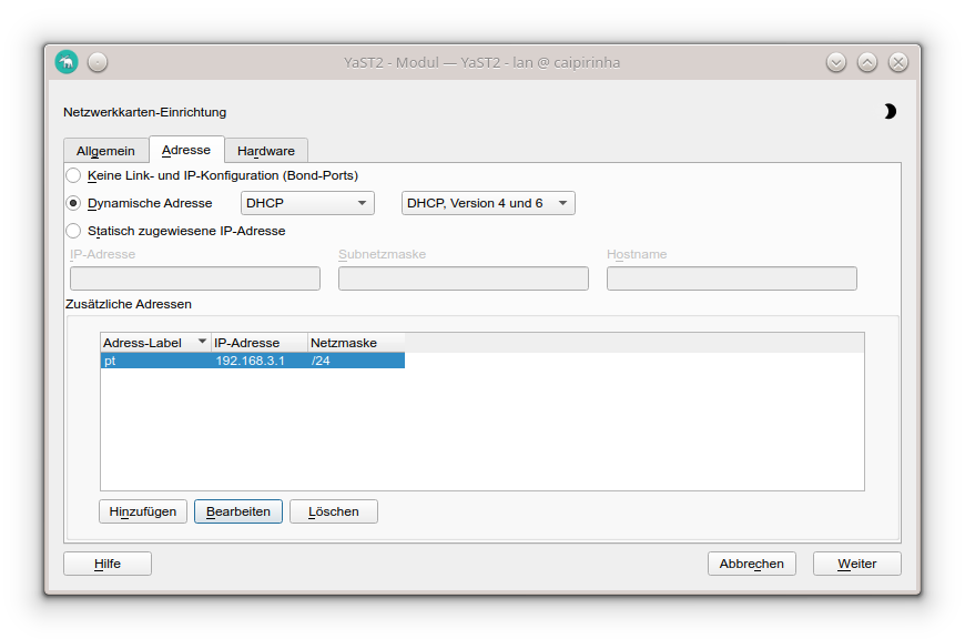
In my case, I chose the address label “pt” (because the original idea was to use this network exclusively for the traffic to Portugal); however, you can choose any label that you wish. While the Linux server usually receives a pseudo-static IP address (192.168.2.3) in the SoHo network 192.168.2.0/24 by the SoHo router (a FRITZ!Box), in our new network 192.168.3.0/24, the server gets the static IP address (192.168.3.1). Clients in this network will consequently require a static IP address configuration; we cannot use DHCP as this network runs on the same physical network infrastructure as the SoHo network 192.168.2.0/24 which already has the FRITZ!Box as DHCP master. In my case, I therefore have configured the TV set (the only client in the network 192.168.3.0/24) with the setup:
- IP address: 192.168.3.186
- Netmask: 255.255.255.0
- Gateway: 192.168.3.1
- DNS server: 192.168.3.1
As DNS I have used the server itself as I have a DNS relay running on the Linux server. If that was not the case, I could also have used 192.168.2.1 which is the address of the FRITZ!Box.
Local WLAN (WiFi) for wireless devices
For the WLAN (WiFi) network I have equipped the Linux server with a PCI Express WLAN card (in my case an old Asus PCE-N10, but I would recommend you a newer one in the 5 GHz band) and attached an external antenna to it. This WiFi card shall act as access point (master). I did not succeed to make that work with YaST2 in conjunction with WPA encryption, and subsequent to my failure, I consulted an Artificial Intelligence (AI) that recommended me to use the package hostapd which needs to be installed on the Linux server. I did so, and after some research and experiments, I came up with a suitable configuration:
/etc/hostapd.conf
# Basis-Einstellungen
interface=wlan0
driver=nl80211
ssid=Querstrasse 8 [BR]
hw_mode=g
channel=1                        # 1-13, vermeiden Sie DFS-Kanäle (52+)
ieee80211n=0                     # Optional für bessere Phones, aber ungünstig bei schlechter Verbindung

# WPA2-PSK (wpa=2 für WPA2 only, TKIP/CCMP für Kompatibilität)
wpa=2
wpa_passphrase=my_secret_password
wpa_key_mgmt=WPA-PSK WPA-PSK-SHA256
wpa_pairwise=TKIP CCMP
rsn_pairwise=CCMP

# Sonstiges
macaddr_acl=0                    # MAC address -based authentication nicht aktivieren
auth_algs=1                      # Open System Authentication
ignore_broadcast_ssid=0          # SSID frei sichtbar
wmm_enabled=0                    # WMM deaktiviert wegen schlechter Verbindung
beacon_int=75                    # Häufigere Beacons wegen schlechter Verbindung
max_num_sta=10                   # Max Clients
country_code=DE
country3=0x49                    # Indoor environment
ieee80211d=1                     # Advertise country-specific parameters
access_network_type=0            # Private network
internet=1                       # Network provides connectivity to the Internet
venue_group=7                    # 7,1 means Private Residence
venue_type=1
ipaddr_type_availability=10      # Double NATed private IPv4 address
logger_syslog=-1
logger_syslog_level=3            # Notifications only
logger_stdout=-1
logger_stdout_level=2
A couple of points in this configuration are important and shall be briefly discussed:
- The network is quite weak in some parts of my house, and so some parameters have been configured for bad network conditions. If you do not have this issue and see a strong WiFi signal all over your place, you might want to change some of the parameters or not set them to dedicated values at all. Consult the original hostapd.conf file for an explanation of all parameters or ask the AI for a suitable setup.
- my_secret_password has to be replaced with the password that you intend to secure your WiFi with, of course.
- I configured the card for Germany, and hence power output is limited to 100 mW, according to the local regulations. A configuration for the USA would allow a higher power output, but this is illegal in Europe. Furthermore, that would only bring a real benefit if your client devices also had higher output power.
- I chose the SSID Querstrasse 8 [BR] (Yes, with white space in the SSID!). If you have old clients, you might want to avoid white spaces in the SSID name.
- I set the values for venue_group, venue_type and access_network_type in order to indicate to prospective clients that this is a private (non-public) network. You might also leave these configuration options away, there would be no real impact.
In order to bring the interface wlan0 to life, we need to issue these three commands:
ip addr add 192.168.4.1/24 dev wlan0
ip link set wlan0 up
systemctl start hostapd.service
However, before we can connect new clients to this WiFi, we need to set up a DHCP server on this network. The small DHCP and DNS caching server dnsmasq is the right tool to be used here.
Providing DHCP and DNS on wlan0
dnsmasq can provide both DHCP as well as cache DNS. That is very practical as it allows us for example, to have only DNS on eth0 where the FRITZ!Box already is the DHCP master, but to configure both DHCP and a caching DNS on wlan0. The following configuration file will exactly do that (it uses only a subset of the capabilities of dnsmasq):
/etc/dnsmasq.conf
# Never forward addresses in the non-routed address spaces.
bogus-priv

# If you don't want dnsmasq to read /etc/resolv.conf or any other
# file, getting its servers from this file instead (see below), then
# uncomment this.
no-resolv

# If you don't want dnsmasq to poll /etc/resolv.conf or other resolv
# files for changes and re-read them then uncomment this.
no-poll

# Add other name servers here, with domain specs if they are for
# non-public domains.
server=8.8.8.8
server=8.8.4.4
server=9.9.9.9
server=1.1.1.1

# If you want dnsmasq to listen for DHCP and DNS requests only on
# specified interfaces (and the loopback) give the name of the
# interface (eg eth0) here.
# Repeat the line for more than one interface.
interface=eth0
interface=wlan0

# If you want dnsmasq to provide only DNS service on an interface,
# configure it as shown above, and then use the following line to
# disable DHCP and TFTP on it.
no-dhcp-interface=eth0

# Uncomment this to enable the integrated DHCP server, you need
# to supply the range of addresses available for lease and optionally
# a lease time. If you have more than one network, you will need to
# repeat this for each network on which you want to supply DHCP
# service.
dhcp-range=tag:wlan0,192.168.4.10,192.168.4.254,24h

# Set the NTP time server addresses
dhcp-option=option:ntp-server,192.168.2.3

# Send Microsoft-specific option to tell windows to release the DHCP lease
# when it shuts down. Note the "i" flag, to tell dnsmasq to send the
# value as a four-byte integer - that's what Microsoft wants. See
# https://learn.microsoft.com/en-us/openspecs/windows_protocols/ms-dhcpe/4cde5ceb-4fc1-4f9a-82e9-13f6b38d930c
dhcp-option=vendor:MSFT,2,1i

# Include all files in a directory which end in .conf
conf-dir=/etc/dnsmasq.d/,*.conf
In this configuration, we can see that on eth0, we will not enable DHCP (Option no-dhcp-interface=eth0). As this option is missing for wlan0, we will have DHCP active on wlan0. Furthermore, we propagate the server’s address 192.168.2.3 as NTP server. For this, the NTP service needs to be enabled, of course, otherwise that would be pointless.
While address 192.168.2.3 is not in the network of wlan0 (192.168.4.0/24), we will enable access to that network in the subsequent chapter.
dnsmasq uses the file /etc/hosts as well as upstream DNS servers for its own DNS service. The advantage of this is that – if your file /etc/hosts is maintained – you can also use the device names listed there. As pstream DNS servers from which dnsmasq gets the IP resolution, I have configured four popular ones (8.8.8.8, 8.8.4.4, 9.9.9.9, 1.1.1.1), but you could also just list the IP of your SoHo router or DNS resolver of your internet provider.
Setting the Routing Policy
Now, we must ensure that traffic from our new networks 192.168.3.0/24 and 192.168.4.0/24 can flow as intended. We have to set up the correct routing policy, and for that, we need the following commands whereby the first three commands have already been mentioned (and been executed) in one of the chapters above:
# Start interfaces wlan0
ip addr add 192.168.4.1/24 dev wlan0
ip link set wlan0 up
systemctl start hostapd.service

# Setup the NAT table for the VPNs.
iptables -t nat -F
iptables -t nat -A POSTROUTING -s 192.168.3.0/24 -o eth0 -j SNAT --to-source 192.168.2.3
iptables -t nat -A POSTROUTING -s 192.168.4.0/24 -o eth0 -j SNAT --to-source 192.168.2.3
iptables -t nat -A POSTROUTING                   -o tun0 -j MASQUERADE
iptables -t nat -A POSTROUTING                   -o tun1 -j MASQUERADE


# Add the missing routes in the other routing tables
for TABLE in Portugal Brasilien; do
    ip route add 192.168.2.0/24 dev eth0  proto kernel scope link src 192.168.2.3 table ${TABLE}
    ip route add 192.168.3.0/24 dev eth0  proto kernel scope link src 192.168.3.1 table ${TABLE}
    ip route add 192.168.4.0/24 dev wlan0 proto kernel scope link src 192.168.4.1 table ${TABLE}
done

# Setup the MANGLE tables which shape and mark the traffic that shall use other routing tables
iptables -t mangle -F
iptables -t mangle -A PREROUTING                            -j CONNMARK --restore-mark
iptables -t mangle -A PREROUTING -m mark  ! --mark 0        -j ACCEPT
iptables -t mangle -A PREROUTING -i eth0  -s 192.168.3.0/24 -j MARK --set-mark 1
iptables -t mangle -A PREROUTING -i wlan0 -s 192.168.4.0/24 -j MARK --set-mark 2
iptables -t mangle -A PREROUTING                            -j CONNMARK --save-mark
iptables -t mangle -A OUTPUT                                -j CONNMARK --restore-mark
iptables -t mangle -A OUTPUT     -m mark  ! --mark 0        -j ACCEPT
iptables -t mangle -A OUTPUT                                -j CONNMARK --save-mark

# Add rules for the traffic that shall branch to the new routing table
ip rule add from all fwmark 0x1 priority 5000 lookup Portugal
ip rule add from all fwmark 0x2 priority 5000 lookup Brasilien
Personally, I have these commands executed as part of a shell script that runs after powering up the Linux server and that I also use to control many other services and configurations.
Once we have started the dnsmasq service (systemctl start dnsmasq.service) from the previous chapter and set up the routing policy correctly, we should be able to connect with a smartphone or a notebook to our new WiFi network 192.168.4.0/24 and do first tests like shown here:


Relocating the TV Set to DE, PT, BR
As a means of convenience, we want to set up a small web page that can be accessed on our smartphone so that we can “re-locate” the TV set between the countries Germany, Portugal, and Brazil. This simple “no frills” page will serve our purpose:
relocate.php:
<!DOCTYPE HTML PUBLIC "-//W3C//DTD HTML 4.0 Transitional//EN">
<html>
<head>
  <title>TV Geo-Relocation</title>
  <style type="text/css">
    a:link { text-decoration:underline; font-weight:normal; color:#0000FF; }
    a:visited { text-decoration:underline; font-weight:normal; color:#800080; }
    a:hover { text-decoration:underline; font-weight:normal; color:#909090; }
    a:active { text-decoration:blink; font-weight:normal; color:#008080; }
    h1 { font-family:Arial,Helvetica,sans-serif; font-size:100%; color:maroon; text-indent:0.0cm; }
    hr { text-indent:0.0cm; height:3px; width:100%; text-align:left; }
    p { font-family:Arial,Helvetica,sans-serif; font-size:80%; color: black; text-indent:0.0cm; }
    body { font-family: Arial, sans-serif; background-color:#FFFFD8; max-width: 600px; margin: 50px auto; padding: 20px; }
    .flag { width: 24px; height: 16px; vertical-align: middle; margin-right: 10px; }
    .radio-group { margin: 20px 0; }
    input[type="radio"] { margin-right: 5px; }
    button { padding: 10px 20px; margin: 10px; background: #007cba; color: white; border: none; cursor: pointer; }
  </style>
  <meta name="viewport" content="width=device-width, initial-scale=1.0">
  <meta http-equiv="content-language" content="de">
  <meta http-equiv="cache control" content="no-cache">
  <meta http-equiv="pragma" content="no-cache">
  <meta name="author" content="Gabriel Rüeck">
  <meta name="date" content="2026-02-17T18:00:00+01:00">
  <meta name="robots" content="noindex">
</head>

<body bgcolor="seashell">
  <?php
    // Setze die neue Markierung für Pakete aus 192.168.3.0/24
    if ($_SERVER['REQUEST_METHOD'] === 'POST') {
      $fwmark = $_POST['fwmark'] ?? '';
      if (in_array($fwmark, ['0','1','2'], true)) {
        shell_exec('sudo /srv/www/htdocs/tv/write_status.sh ' . escapeshellarg($fwmark));
      }
    }

    // Hole aktuelle Markierung für Pakete aus 192.168.3.0/24
    $current_mark = trim(shell_exec('sudo /srv/www/htdocs/tv/read_status.sh'));
  ?>
  <h1>TV Geo-Relocation</h1>

  <form method="POST">
    <div class="radio-group">
      <label>
        <input type="radio" name="fwmark" value="0" <?= $current_mark === '0x0' ? 'checked' : '' ?>>
        <img src="https://flagcdn.com/24x18/de.png" srcset="https://flagcdn.com/48x36/de.png 2x" class="flag" alt="🇩🇪"> Deutschland (0x0)
      </label><br><br>

      <label>
        <input type="radio" name="fwmark" value="1" <?= $current_mark === '0x1' ? 'checked' : '' ?>>
        <img src="https://flagcdn.com/24x18/pt.png" srcset="https://flagcdn.com/48x36/pt.png 2x" class="flag" alt="🇵🇹"> Portugal (0x1)
      </label><br><br>

      <label>
        <input type="radio" name="fwmark" value="2" <?= $current_mark === '0x2' ? 'checked' : '' ?>>
        <img src="https://flagcdn.com/24x18/br.png" srcset="https://flagcdn.com/48x36/br.png 2x" class="flag" alt="🇧🇷"> Brasilien (0x2)
      </label>
    </div>

    <button type="submit">Anwenden</button>
    <button type="button" onclick="location.reload()">Neu laden</button>

    <p>Flags with courtesy from <a href="https://flagpedia.net" target="_blank">flagpedia.net</a>.</p>
  </form>

</body>
</html>
This PHP page needs to be put in a suitable directory, and you need to have web server up and running, of course (not described in this article). In my case, the file is located in /srv/www/htdocs/tv/relocate.php. In the header of the PHP file, you can see the line:
<meta name="viewport" content="width=device-width, initial-scale=1.0">This line adapts the width of the page when being called on a smartphone so that it appears with a reasonable scaling on the smartphone screen. Furthermore, as you can see, this web page calls two shell scripts, and those are:
read_status.sh
#! /bin/bash
#
# This script will be executed as root by the PHP scipt relocate.php
#
# Gabriel Rüeck 15.02.2026
#

/usr/sbin/iptables -t mangle --line-numbers -L PREROUTING -n -v | fgrep "eth0" | sed -r 's/^.*MARK (set|and) (0x[[:xdigit:]]+)/\2/'
write_status.sh
#! /bin/bash
#
# This script will be executed as root by the PHP scipt relocate.php
#
# Gabriel Rüeck 15.02.2026
#

LINE_NUMBER=$(/usr/sbin/iptables -t mangle --line-numbers -L PREROUTING -n -v | fgrep "eth0" | sed 's/^\([[:digit:]]\+\) \+.*/\1/')
MARK=${1}
/usr/sbin/iptables -t mangle -R PREROUTING ${LINE_NUMBER} -i eth0 -s 192.168.3.0/24 -j MARK --set-mark ${MARK}
read_status.sh reads the corresponding routing entry from the mangle table [6], and this information enables the page relocate.php to display the correct country to which the traffic of the TV set if channeled when relocate.php is called initially. write_status.sh is used to modify the correct entry in the mangle table and channel the traffic to the country select on the PHP page. Both read_status.sh as well as write_status.sh need to be executed as root, and therefore, they need to be listed in the sudoers file structure. [7], [8] explain the correct proceeding. In our case, the file /etc/sudoers.d/wwwrun has been set up with the access rights 0440, and this file should have the content:
wwwrun ALL=(root) NOPASSWD: /srv/www/htdocs/tv/read_status.sh
wwwrun ALL=(root) NOPASSWD: /srv/www/htdocs/tv/write_status.sh
Of course, we do not want arbitrary internet users to change the geo-location of the TV set, and therefore, the access to the PHP page relocate.php must be restricted. An easy, but not entirely secure method is to limit access to this page to the local networks. This can be done in the webserver configuration file (in my case: /etc/apache2/httpd.conf.local) where we add:
# TV Configuration
<Directory /srv/www/htdocs/tv>
  Require local
  Require ip 192.168.0.0/16 127.0.0.0/8 ::1/128 fd00:0:0::/48
</Directory>
This will restrict access to local networks. But this is entirely fool-proof against advanced hacking attacks (see [9] as an example).
The PHP page should ultimately look like this on a smartphone:

Shortcomings
During experiments with this setup, I have come across the following shortcoming:
- On my TV set, a Samsung GQ75Q80, I was able to configure a static IPv4 address. However, it seemed to me that the TV was still getting a dynamic IPv6 address from the FRITZ!Box. I suppose that if one really wants to isolate the TV set from the SoHo network, it would be necessary to use a separate physical network. Luckily, this did not impact the possibility to watch TV with the Portuguese TV app.
Conclusion
With Policy Routing and commercial VPN connections, it is possible to create additional networks in a SoHo environment that will allow client devices to behave as if they were in another country. Basically, you could also achieve that with a VPN connection on the device (smartphone, etc.) itself; however, you then might have access to other services in your SoHo network (printer, etc.). And in the case of a TV set, I am not even sure if there are models that can build up VPN connections themselves. However, the setup described here also shows that it is not trivial as several services need to be configured and act together in a meaningful way.
Sources
- [1] = Setting up Client VPNs, Policy Routing
- [2] = Setting up Dual Stack VPNs
- [3] = iptables – Port forwarding over OpenVpn
- [4] = Routing for multiple uplinks/providers
- [5] = Two Default Gateways on One System
- [6] = Netfilter
- [7] = Classic SysAdmin: Configuring the Linux Sudoers File
- [8] = How To Edit the Sudoers File Safely
- [9] = Forcepoint Research Report: Attacking the internal network from the public Internet using a browser as a proxy
Protected: Road Trip nach Portugal (II)
Learnings from Dynamic Electricity Pricing
Executive Summary
Unlike previous articles, I chose to split this new blog post into two parts. In the first part (Findings), I will elaborate on my findings as a consumer with dynamic electricity prices (day-ahead market) in connection with a small solar electricity generation unit. We will look at various visualizations that help to understand the impact and to gain some more insight in how dynamic electricity prices can be useful. In the second part (Annex: Technical Details), technically interested folks will find the respective queries and sample data with which they can replicate the findings or even do their own examination with the sample data. As in previous articles, Grafana is used in connection with a MariaDB database.
Background
On 1st of March 2024, I switched from a traditional electricity provider to one with dynamic day-ahead pricing, in my case, Tibber. I wanted to try this contractual model and see if I could successfully manage to shift chunks of high electricity consumption such as:
- … loading the battery-electric vehicle (BEV) or the plug-in hybrid car (PHEV)
- … washing clothes
- … drying clothes in the electric dryer
to those times of the day when the electricity price is lower. I also wanted to see if that makes economic sense for me. And, after all, it is fun to play around with data and gain new insights.
As my electricity supplier, I had chosen Tibber because they were the first one I got to know and they offer a device called Pulse which can connect a digital electricity meter to their infrastructure for metering and billing purposes. Furthermore, they do have an API [1] which allows me to read out my own data; that was very important for me. I understand that meanwhile, there are several providers Tibber that have similar models and comparable features.
Findings
Price and consumption patterns
The graph below shows five curves and is an upgraded version of the respective graph in [6] visualizing data over two weeks:
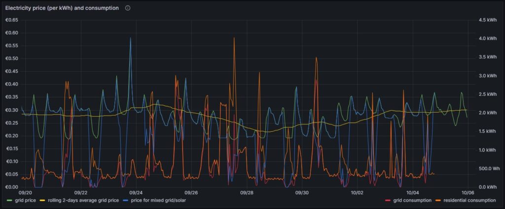
As in [6], the green curve is the hourly price of the day-ahead market. It is well recognizable that the price has peaks in the evening and in the morning at breakfast time when residential consumption is high, but little solar energy is available in Germany. The yellow curve is a two-days floating average and shows that the average price is not below a fixed rate electricity contract, an important point that we shall discuss later. The orange curve is the consumption of my house; the higher peaks indicate times when I charged one of the cars using an ICCB (one phase, current: 10 A). The red curve shows the consumption of the grid. During the day, when there is sunshine, the red curve lies below the orange curve as a part of the overall consumed electricity comes from the solar panels. At nighttime, the red curve will exactly lie on the orange curve as there is no solar electricity generation. The blue curve shows the average electricity price per kWh based on a mixed calculation of the grid price and zero for my own solar electricity generation. One might argue whether zero is an adequate assumption as also solar panels cost money, but as I do have them installed already, I consider them to be sunk cost now. The blue curve show an interesting behavior: When my consumption is low, the blue curve shows a small average price. When the consumption of the house is less than the power that is generated by the solar panels, then the blue curve is flat zero. When, however, I consume a lot of power, then, the blue curve approaches the green curve. At nighttime when there is no solar energy generation, the blue curve lies identical with the green curve.
My goal is to consume more electricity in the times when either the green curve points to a low electricity price or when there is enough electricity generated by the solar panels so that my average price that I pay (blue curve) is reasonable low. This also explains why I mostly the ICCB (one phase, 10 A) to charge the cars as then, I still can get a good average price (although charging takes a lot more time then). I think that by looking at the curves, I have adapted my consumption pattern well to the varying electricity price.
Actual cost, minimal cost, maximal cost, average cost per day
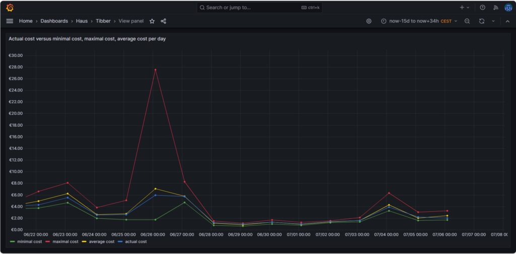
The graph above shows four curves. The green curve is the cost that I would have incurred if I had bought all the electricity of the respective day in the hour of the cheapest electricity price. This would only be possible if I had a battery that could bridge the remaining 23 hours of the day (and probably some hours more as the cheapest hour of the following day is not necessarily 00:00-01:00). The red curve is the cost that I would have incurred if I had bought all the electricity of the respective day in the hour of the most expensive electricity price. The yellow curve is the average cost of the respective day, the multiplication of the average price per kWh of that day by my consumed energy. The blue curve is the real cost that I have paid. If the blue curve is between the yellow curve and the green curve, then this is very good, and I have succeeded in shifting my consumption versus the hours with cheaper electricity. Without a battery, it is almost impossible to come very close to the green line.
The graph above shows one peculiarity as on 2024-06-26, there were some hours with an extremely high price, but that was due to a communication error that decoupled the auction in Germany from the rest of Europe [7], clearly (and hopefully) a one-time event.
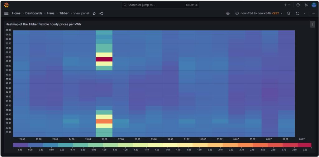
Price heatmap of the hourly prices per kWh
The one-time event with unusually high prices [7] is well visible in the price heatmap that was already introduced and explained in [6]. The one-time event overshadows all price fluctuations in the rest of the week.
Cost and amount of purchased electricity from grid with price indication
The first graph shown below was already introduced and explained in [6] and shows the cost of purchased electricity from the grid in 24 rectangles, whereby each rectangle represents an hour. The order of the rectangles starts with the most expensive hour at the top and ends with the least expensive hour at the bottom. The larger the rectangle, the more money has been spent in the respective hour. I already explained in [6] that the goal should be – if electricity has to be purchased from the grid at all – the purchases ideally should happen in times when the price is low. In the graph those are the rectangles with green or at maximum yellow color. The rectangles with orange and red color indicate purchases during times of a high electricity price. In reality, one will not be able to avoid purchases at times of a high price completely. My experience is that in summer, I let the air conditioning systems run also in the evening hours when the electricity price is higher, just to keep the house at reasonable temperatures inside. Similarly, in spring and autumn, I opt for leaving the central heating switched off and try to heat the rooms in which I am usually with the air conditioning systems (in heating mode) as in spring and autumn, the difference in temperature between outside and inside is not too high, and the air conditioning systems will have a high efficiency.
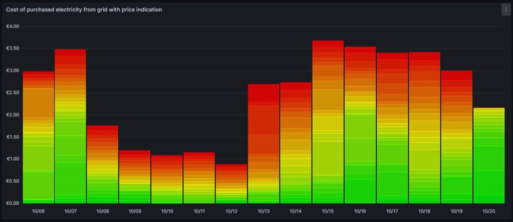
Then, for 13-Oct (10/13), one can see that in fact I bought substantial electricity at high prices. The reason for that was that I returned home at night and had to re-charge the car for the next day. So, one cannot always avoid purchasing electricity at high prices.
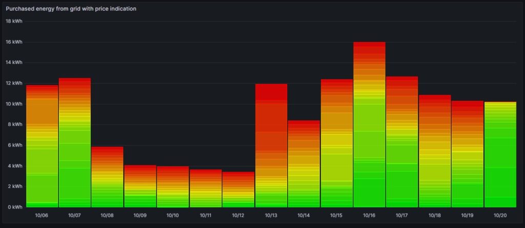
The next chart offers another view on the same topic. Rather than looking at the cost of the purchased electricity, we look at the amount of purchased electricity. This offers an interesting insight. Except for 13-Oct, the amount of electricity that is purchased at hours with a high price, is less than 5 kWh. This means that with an energy-storage system (ESS), it should be possible to charge a battery of around 5 kWh during times of a lower electricity price and to discharge the battery and supply the house during times of a high electricity price so that ideally, there would be no or only minimally sized orange and red rectangles. Of course, this only makes sense if the low prices and the high prices per day differ substantially as the ESS will have losses of 10%…20%. And in fact, this is exactly an idea that I am planning to try out within the next months (so stay tuned).
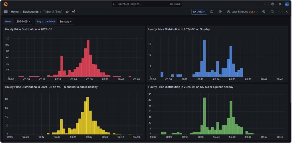
Hourly price distribution
Another finding which was interesting for me was that the price of electricity is not necessarily cheaper on the weekend (at least not in May 2024). One might assume that because industry consumption is low on the weekend, the price of electricity is lower. And that is true to some parts, as the lowest prices that occur within a whole month tend to happen on the weekend (green histogram). We can also see a peak at around 19 ¢/kWh in the green histogram which is much lower in the yellow histogram. However, there are also many hours with prices that are similar to the prices that we have during the week (yellow histogram).
Monthly hourly price curves
The following three graphs show the hourly price curves over the hour of the day per month; the selected Day of the Week is irrelevant for this graph as only the variable Month is used.
The green curve shows the minimum hourly price per kWh that occurred in the selected month. The red curve shows the maximum hourly price per kWh that occurred in the selected month. The yellow curve shows the average hourly price per kWh that occurred in the selected month. The blue curve shows the average hourly price per kWh that I have experienced in the selected month, calculating my own solar electricity generation as “free of cost” (like the blue curve of the graph in chapter Price and consumption patterns).
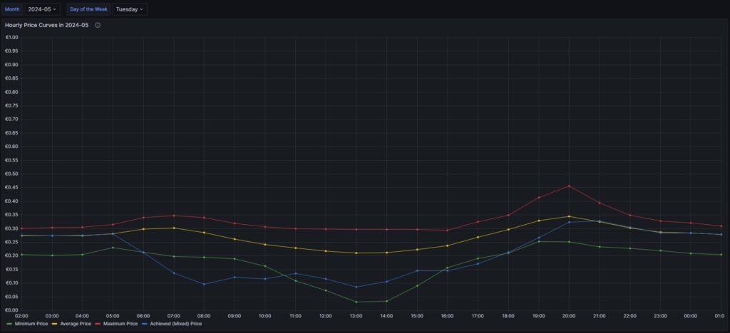
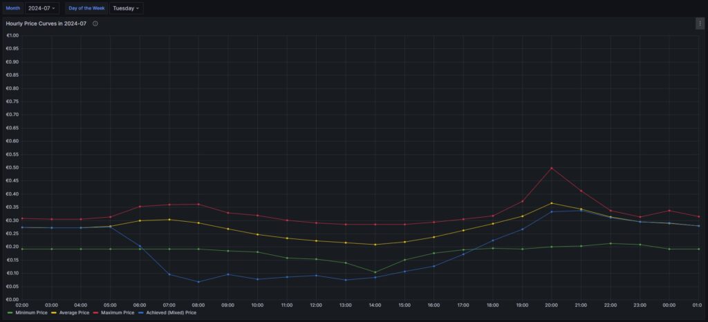
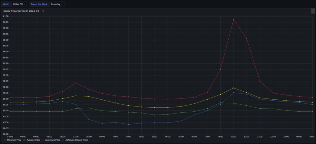
There are a couple of interesting findings that can easily be seen in the curves:
- Prices tend to be higher in the early morning (06:00-08:00) and in the evening (18:00-21:00). The evening price peak is higher than the one in the morning.
- The price gap in the morning, but especially in the evening hours between the minimum and the maximum hourly price seems to increase from May to September. I do not yet know if this is because of the season, or if the market has become more volatile in general.
- In my personal situation (the solar modules face East), I am not bothered by the price peak in the morning, as I seem to have already quite a good power generation (blue curve descending in the morning). That is, however, different in the evening; then, I am personally affected by the price peak.
For me, this is an indication that it might make sense to install a battery and charge it during the day and discharge it especially in the evening hours (18:00-21:00) when the price peaks.
Electricity price levels
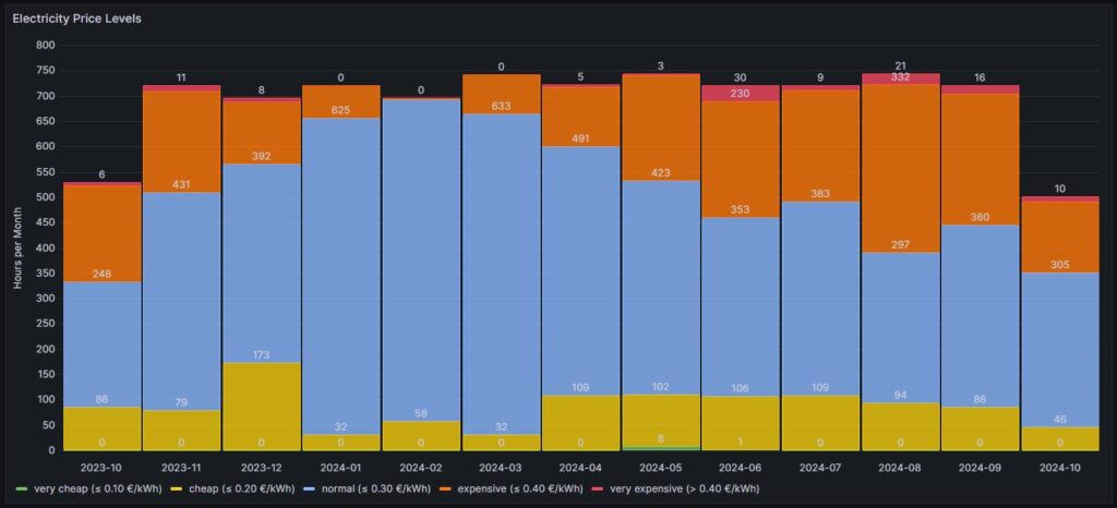
In order to look into the hourly prices from a different perspective, I have grouped the hourly prices into five categories:
- Price per kWh ≤10 ¢/kWh (green block), labelled as very cheap
- Price per kWh >10 ¢/kWh and ≤20 ¢/kWh (yellow block), labelled as cheap
- Price per kWh >20 ¢/kWh and ≤30 ¢/kWh (blue block), labelled as normal
- Price per kWh >30 ¢/kWh and ≤40 ¢/kWh (orange block), labelled as expensive
- Price per kWh >40 ¢/kWh (red block), labelled as very expensive
For each month (except for Oct 2023, Oct 2024) the sum of the blocks in different colors are the hours of the respective month; depending on the number of days per month, the number of hours vary, of course. Larger blocks correspond to more hours in the respective price category. Do not pay attention to the numbers listed in the graph in white color as some numbers are missing. I will give a numerical statistic below the graph.
| Month | very cheap (≤ 10 ¢/kWh) | cheap (≤ 20 ¢/kWh) | normal (≤ 30 ¢/kWh) | expensive (≤ 40 ¢/kWh) | very expensive (> 40 ¢/kWh) |
| 2023-10 | 0 | 86 | 248 | 189 | 6 |
| 2023-11 | 0 | 79 | 431 | 199 | 11 |
| 2023-12 | 0 | 173 | 392 | 123 | 8 |
| 2024-01 | 0 | 32 | 625 | 63 | 0 |
| 2024-02 | 0 | 58 | 635 | 3 | 0 |
| 2024-03 | 0 | 32 | 633 | 78 | 0 |
| 2024-04 | 0 | 109 | 491 | 117 | 5 |
| 2024-05 | 8 | 102 | 423 | 208 | 3 |
| 2024-06 | 1 | 106 | 353 | 230 | 30 |
| 2024-07 | 0 | 109 | 383 | 219 | 9 |
| 2024-08 | 0 | 94 | 297 | 332 | 21 |
| 2024-09 | 0 | 86 | 360 | 258 | 16 |
| 2024-10 | 0 | 46 | 305 | 141 | 10 |
Before I had generated this graph and the ones of the previous chapter, my initial assumption had been that in summer, the prices would go down compared to winter. And to some part, this is true. There is a higher number of hours in the category “cheap” (yellow block). However, the category “expensive” (orange block) increases even more in summer. And even the category “very expensive” (red block) becomes noticeable whereas the category “very cheap” (green block) does not manifest itself, not even in summer. I do not have an explanation for this; my assumption though is that maybe in winter, some fossil power stations are active that are switched off in summer and that therefore, the price is much more susceptible to the change in the electricity offer over the day. I suspect that during the day, there is mostly enough solar electricity generation, and in the evening, gas power stations need to be started that then determine the price level and lead to increased prices. However, I do not have any statistics underpinning this assumption.
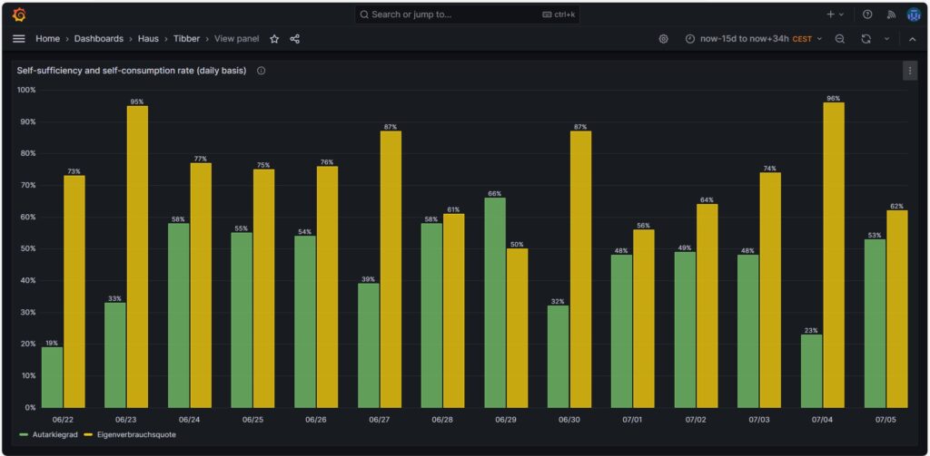
Self-sufficiency (Autarkie) and sef-consumption (Eigenverbrauch)
I am not much of a friend of looking at the values of self-sufficiency (de: Autarkie) and self-consumption (de: Eigenverbrauch), and this is for the following reasons:
- If you do not live in a place where an electricity grid is not available or where the grid is very unreliable, it does not make sense to strive for complete self-sufficiency. It is still economically best if you use your electricity during the day and consume electricity from the grid at night. Similarly, you will probably need to buy electricity from the grid in winter, at least in Central or Northern Europe as in winter, the output from your own solar electricity generation is usually insufficient to power the consumption of your house.
- The value for self-consumption varies strongly with your consumption pattern and with the solar intensity on the respective day. The only conclusion that you can draw from observing the self-consumption values over a longer time frame is:
- If your values are constantly low, then you probably have spent into too large of a solar system.
- If your values are constantly high or 100%, then it might make sense to add some more solar panels to your system.
Nevertheless, for the sake of completion, here are some example values from July of this year.
Conclusion
- The field of dynamic electricity pricing is technically very interesting and certainly helps to sharpen awareness for the need to consume electricity precisely then, when there is a lot of it available.
- Economically, having a dynamic electricity price can make sense under certain conditions. I side with [8] when I say:
- For a household without an electric car or another large electricity consumer, it does not make sense to use dynamic electricity pricing. The consumption of the washing machine, the dryer, and the dishwasher are not large enough to really draw a benefit.
- For a household with an electric car that has a large battery (e.g., some 80+ kWh, unfortunately not my use case), it makes sense then when you have the flexibility to charge the car during times with a low electricity price.
Annex: Technical Details
Preconditions
In order to use the approach described below, you should:
- … have access to a Linux machine or account
- … have a MySQL or MariaDB database server installed, configured, up and running
- … have the package Grafana [2] installed, configured, up and running
- … have the package Node-RED [3] installed, configured, up and running
- … have access to the data of your own electricity consumption and pricing information of your supplier or use the dataset linked below in this blog
- … have some basic knowledge of how to operate in a Linux environment and some basic understanding of shell scripts
- … have read and understood the previous blog post [6], especially the part on how to connect Grafana to the MySQL or MariaDB database server
The Database
The base for the following visualizations is a fully populated MariaDB database with the following structure:
# Datenbank für Analysen mit Tibber
# V2.0; 2024-09-12, Gabriel Rüeck <gabriel@rueeck.de>, <gabriel@caipirinha.spdns.org>
# Delete existing databases
REVOKE ALL ON tibber.* FROM 'gabriel';
DROP DATABASE tibber;

# Create a new database
CREATE DATABASE tibber DEFAULT CHARSET utf8mb4 COLLATE utf8mb4_general_ci;
GRANT ALL ON tibber.* TO 'gabriel';
USE tibber;
SET default_storage_engine=Aria;

CREATE TABLE preise         (uid               INT UNSIGNED NOT NULL PRIMARY KEY AUTO_INCREMENT,\
                             zeitstempel       DATETIME NOT NULL UNIQUE,\
                             preis             DECIMAL(5,4),\
                             niveau            ENUM('VERY_CHEAP','CHEAP','NORMAL','EXPENSIVE','VERY_EXPENSIVE'));

CREATE TABLE verbrauch      (uid               INT UNSIGNED NOT NULL PRIMARY KEY AUTO_INCREMENT,\
                             zeitstempel       DATETIME NOT NULL UNIQUE,\
                             energie           DECIMAL(5,3),\
                             kosten            DECIMAL(5,4));

CREATE TABLE zaehler        (uid               INT UNSIGNED NOT NULL PRIMARY KEY AUTO_INCREMENT,\
                             zeitstempel       TIMESTAMP NOT NULL DEFAULT UTC_TIMESTAMP,\
                             bezug             DECIMAL(9,3) DEFAULT NULL,\
                             erzeugung         DECIMAL(9,3) DEFAULT NULL,\
                             einspeisung       DECIMAL(9,3) DEFAULT NULL);
Data Acquisition
Data for the MariaDB database is acquired with two different methods.
The tables preise and verbrauch are populated with the following bash script. You will need a valid API token of your Tibber account [4]; in this script, you need to replace _API_TOKEN with your personal API token ([4]) and _HOME_ID with your personal Home ID ([1]). The script further assumes that the user gabriel can login to the MySQL database without further authentication; this can be achieved by writing the MySQL login information in the file ~/.my.cnf.
#!/bin/bash
#
# Dieses Skript liest Daten für die Tibber-Datenbank und speichert das Ergebnis in einer MySQL-Datenbank ab.
# Das Skript wird einmal pro Tag aufgerufen.
#
# V2.0; 2024-09-12, Gabriel Rüeck <gabriel@rueeck.de>, <gabriel@caipirinha.spdns.org>
#
# CONSTANTS
declare -r    MYSQL_DATABASE='tibber'
declare -r    MYSQL_SERVER='localhost'
declare -r    MYSQL_USER='gabriel'
declare -r    TIBBER_API_TOKEN='_API_TOKEN'
declare -r    TIBBER_API_URL='https://api.tibber.com/v1-beta/gql'
declare -r    TIBBER_HOME_ID='_HOME_ID'

# VARIABLES

# PROGRAM
# Read price information for tomorrow
curl -s -S -H "Authorization: Bearer ${TIBBER_API_TOKEN}" -H "Content-Type: application/json" -X POST -d  '{ "query": "{viewer {home (id: \"'"${TIBBER_HOME_ID}"'\") {currentSubscription {priceInfo {tomorrow {total startsAt level }}}}}}" }' "${TIBBER_API_URL}" | jq -r '.data.viewer.home.currentSubscription.priceInfo.tomorrow[] | .total, .startsAt, .level' | while read cost; do
  read LINE
  read level
  timestamp=$(echo "${LINE%%+*}" | tr 'T' ' ')
  # Determine timezone offset and store the UTC datetime in the database
  offset="${LINE:23}"
  mysql --default-character-set=utf8mb4 -B -N -r -D "${MYSQL_DATABASE}" -h ${MYSQL_SERVER} -u ${MYSQL_USER} -e "INSERT INTO preise (zeitstempel,preis,niveau) VALUES (DATE_SUB(\"${timestamp}\",INTERVAL \"${offset}\" HOUR_MINUTE),${cost},\"${level}\");"
done

# Read consumption information from the past 24 hours
curl -s -S -H "Authorization: Bearer ${TIBBER_API_TOKEN}" -H "Content-Type: application/json" -X POST -d  '{ "query": "{viewer {home (id: \"'"${TIBBER_HOME_ID}"'\") {consumption (resolution: HOURLY, last: 24) {nodes {from to cost consumption}}}}}" }' "${TIBBER_API_URL}" | jq -r '.data.viewer.home.consumption.nodes[] | .from, .consumption, .cost' | while read LINE; do
  read consumption
  read cost
  timestamp=$(echo "${LINE%%+*}" | tr 'T' ' ')
  # Determine timezone offset and store the UTC datetime in the database
  offset="${LINE:23}"
  mysql --default-character-set=utf8mb4 -B -N -r -D "${MYSQL_DATABASE}" -h ${MYSQL_SERVER} -u ${MYSQL_USER} -e "INSERT INTO verbrauch (zeitstempel,energie,kosten) VALUES (DATE_SUB(\"${timestamp}\",INTERVAL \"${offset}\" HOUR_MINUTE),${consumption},${cost});"
done
The table zaehler is populated via a Node-RED flow that reads data from the Tibber API [4] as well as from the AVM socket FRITZ!DECT 210 and stores new values for the columns bezug, erzeugung, einspeisung every 15 minutes. I used a Node-RED flow for this because otherwise, I would have to program code for the access of the Tibber API [4] and include code [5] for the AVM socket FRITZ!DECT 210. However, I do plan to enlarge the functionality later with an Energy Storage System (ESS) and a battery, and so Node-RED seemed suitable to me. The flow is shown here; it contains some additional nodes apart from the now needed functionality, and it is still in development:
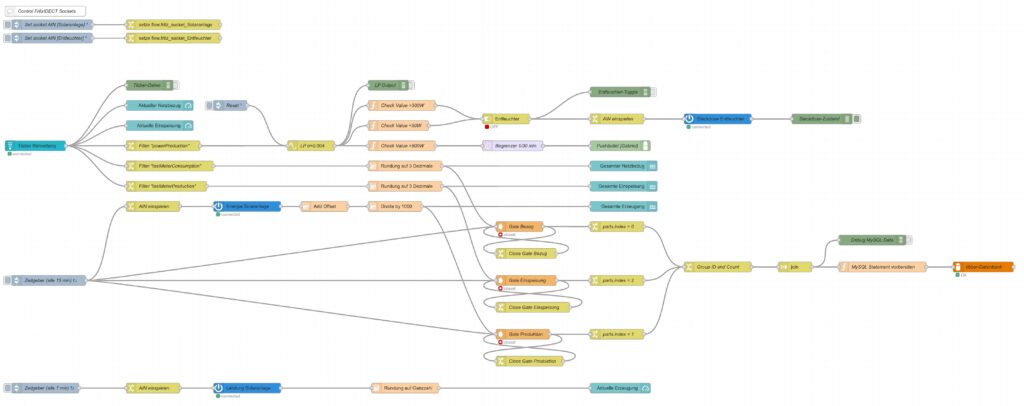
I have decided not to publish the JSON code here as I am not yet entirely familiar with Node-RED [3] and would not know how to remove my personal tokens from the JSON code.
Queries for the Graphs
Price and Consumption Patterns
The graph is based on four queries that correspond to the green and yellow, to the red, to the orange and to the blue curve:
SELECT zeitstempel,
       preis AS 'grid price',
       AVG(preis) OVER (ORDER BY zeitstempel ROWS BETWEEN 47 PRECEDING AND CURRENT ROW) as 'rolling 2-days average grid price'
FROM preise;

SELECT zeitstempel, energie AS 'grid consumption' FROM verbrauch;

SELECT alt.zeitstempel,
       (neu.bezug-alt.bezug+neu.erzeugung-alt.erzeugung-neu.einspeisung+alt.einspeisung) AS 'residential consumption'
FROM zaehler AS neu JOIN zaehler AS alt ON neu.uid=(alt.uid+4)
WHERE MINUTE(alt.zeitstempel)=0;

SELECT alt.zeitstempel,
       ROUND(preise.preis*(neu.bezug-alt.bezug)/(neu.bezug-alt.bezug+neu.erzeugung-alt.erzeugung-neu.einspeisung+alt.einspeisung),4) AS 'price for mixed grid/solar'
FROM zaehler AS neu
JOIN zaehler AS alt ON neu.uid=(alt.uid+4)
LEFT JOIN preise ON DATE_FORMAT(preise.zeitstempel, "%Y%m%d%H%i")=DATE_FORMAT(alt.zeitstempel, "%Y%m%d%H%i")
WHERE MINUTE(alt.zeitstempel)=0
  AND preise.zeitstempel>=DATE_SUB(CURRENT_DATE(),INTERVAL 30 DAY);
Actual cost, minimal cost, maximal cost, average cost per day
This graph uses only one query:
SELECT DATE(preise.zeitstempel) AS 'date',
       MIN(preise.preis)*SUM(verbrauch.energie) AS 'minimal cost',
       MAX(preise.preis)*SUM(verbrauch.energie) AS 'maximal cost',
       AVG(preise.preis)*SUM(verbrauch.energie) AS 'average cost',
       SUM(verbrauch.kosten) AS 'actual cost'
FROM preise JOIN verbrauch ON verbrauch.zeitstempel=preise.zeitstempel
WHERE DATE(preise.zeitstempel)>'2024-03-03'
GROUP BY DATE(preise.zeitstempel);
Cost and amount of purchased electricity from grid with price indication
The first graph (Cost of purchased electricity from grid with price indication) uses the query:
SELECT DATE_FORMAT(preise.zeitstempel,'%m/%d') AS 'Datum',
       ROW_NUMBER() OVER (PARTITION BY DATE(preise.zeitstempel) ORDER BY preise.preis ASC) AS 'Row',
	   verbrauch.kosten AS 'Kosten'
FROM preise JOIN verbrauch ON verbrauch.zeitstempel=preise.zeitstempel
WHERE DATE(preise.zeitstempel)>DATE_ADD(CURDATE(), INTERVAL -15 DAY)
ORDER BY DATE(preise.zeitstempel) ASC, preise.preis ASC;
The second graph (Amount of purchased electricity from grid with price indication) uses the query:
SELECT DATE_FORMAT(preise.zeitstempel,'%m/%d') AS 'Datum',
       ROW_NUMBER() OVER (PARTITION BY DATE(preise.zeitstempel) ORDER BY preise.preis ASC) AS 'Row',
	   verbrauch.energie AS 'Energie'
FROM preise JOIN verbrauch ON verbrauch.zeitstempel=preise.zeitstempel
WHERE DATE(preise.zeitstempel)>DATE_ADD(CURDATE(), INTERVAL -15 DAY)
ORDER BY DATE(preise.zeitstempel) ASC, preise.preis ASC;
Hourly price distribution
The red histogram uses the query:
SELECT preis FROM preise WHERE DATE_FORMAT(zeitstempel,'%Y-%m')='${Month}';The blue histogram uses the query:
SELECT preis FROM preise
WHERE DATE_FORMAT(zeitstempel,'%Y-%m')='${Month}'
  AND DAYNAME(zeitstempel)='${Weekday}';
The yellow histogram uses the query:
SELECT preis FROM preise
WHERE DATE_FORMAT(zeitstempel,'%Y-%m')='${Month}'
  AND WEEKDAY(zeitstempel)<5
  AND DATE(zeitstempel) NOT IN (SELECT datum FROM aux_feiertage);
The green histogram uses the query:
SELECT preis FROM preise
WHERE DATE_FORMAT(zeitstempel,'%Y-%m')='${Month}'
  AND WEEKDAY(zeitstempel)>=5
  OR DATE(zeitstempel) IN (SELECT datum FROM aux_feiertage WHERE DATE_FORMAT(zeitstempel,'%Y-%m')='${Month}');
The tables use these variables on the respective Grafana dasboard as well as the additional helper table aux_feiertage (indicating national holidays) in the MariaDB database.
The variable Month on the Grafana dasboard has the query:
SELECT DISTINCT(DATE_FORMAT(zeitstempel,'%Y-%m')) FROM preise;The variable Weekday on the Grafana dasboard has the query:
SELECT aux_wochentage.wochentag AS Weekday
FROM aux_wochentage JOIN aux_sprachen ON aux_sprachen.id_sprache=aux_wochentage.id_sprache
WHERE aux_sprachen.sprachcode='en'
ORDER BY aux_wochentage.id_tag ASC;
The last query also uses the tables aux_wochentage and aux_sprachen in order to offer a multi-lingual interface (not really necessary for the functionality). The tables are:
CREATE TABLE aux_wochentage (id_tag            TINYINT UNSIGNED NOT NULL,\
                             id_sprache        TINYINT UNSIGNED NOT NULL,\
                             wochentag         VARCHAR(30) NOT NULL);

CREATE TABLE aux_sprachen   (id_sprache        TINYINT UNSIGNED NOT NULL PRIMARY KEY,\
                             sprachcode        CHAR(2),\
                             sprache           VARCHAR(30));

CREATE TABLE aux_feiertage  (uid               SMALLINT UNSIGNED NOT NULL PRIMARY KEY AUTO_INCREMENT,\
                             datum             DATE NOT NULL,\
                             beschreibung      VARCHAR(50));

INSERT INTO aux_sprachen   VALUES (0,'en','English'),\
                                  (1,'de','Deutsch'),\
                                  (2,'pt','Português'),\
                                  (3,'zh','中文');

INSERT INTO aux_wochentage VALUES (0,0,'Monday'),\
                                  (1,0,'Tuesday'),\
                                  (2,0,'Wednesday'),\
                                  (3,0,'Thursday'),\
                                  (4,0,'Friday'),\
                                  (5,0,'Saturday'),\
                                  (6,0,'Sunday'),\
                                  (0,1,'Montag'),\
                                  (1,1,'Dienstag'),\
                                  (2,1,'Mittwoch'),\
                                  (3,1,'Donnerstag'),\
                                  (4,1,'Freitag'),\
                                  (5,1,'Samstag'),\
                                  (6,1,'Sonntag'),\
                                  (0,2,'segunda-feira'),\
                                  (1,2,'terça-feira'),\
                                  (2,2,'quarta-feira'),\
                                  (3,2,'quinta-feira'),\
                                  (4,2,'sexta-feira'),\
                                  (5,2,'sábado'),\
                                  (6,2,'domingo'),\
                                  (0,3,'星期一'),\
                                  (1,3,'星期二'),\
                                  (2,3,'星期三'),\
                                  (3,3,'星期四'),\
                                  (4,3,'星期五'),\
                                  (5,3,'星期六'),\
                                  (6,3,'星期日');

INSERT INTO aux_feiertage (datum, beschreibung) VALUES ('2023-01-01','Neujahr'),\
                               ('2023-01-06','Heilige Drei Könige'),\
                               ('2023-04-07','Karfreitag'),\
                               ('2023-04-10','Ostermontag'),\
                               ('2023-05-01','Tag der Arbeit'),\
                               ('2023-05-18','Christi Himmelfahrt'),\
                               ('2023-05-29','Pfingstmontag'),\
                               ('2023-06-08','Fronleichnam'),\
                               ('2023-08-15','Mariä Himmelfahrt'),\
                               ('2023-10-03','Tag der Deutschen Einheit'),\
                               ('2023-11-01','Allerheiligen'),\
                               ('2023-12-25','1. Weihnachtstag'),\
                               ('2023-12-26','2. Weihnachtstag'),\
                               ('2024-01-01','Neujahr'),\
                               ('2024-01-06','Heilige Drei Könige'),\
                               ('2024-03-29','Karfreitag'),\
                               ('2024-04-01','Ostermontag'),\
                               ('2024-05-01','Tag der Arbeit'),\
                               ('2024-05-09','Christi Himmelfahrt'),\
                               ('2024-05-20','Pfingstmontag'),\
                               ('2024-05-30','Fronleichnam'),\
                               ('2024-08-15','Mariä Himmelfahrt'),\
                               ('2024-10-03','Tag der Deutschen Einheit'),\
                               ('2024-11-01','Allerheiligen'),\
                               ('2024-12-25','1. Weihnachtstag'),\
                               ('2024-12-26','2. Weihnachtstag'),\
                               ('2025-01-01','Neujahr'),\
                               ('2025-01-06','Heilige Drei Könige'),\
                               ('2025-04-18','Karfreitag'),\
                               ('2025-04-21','Ostermontag'),\
                               ('2025-05-01','Tag der Arbeit'),\
                               ('2025-05-29','Christi Himmelfahrt'),\
                               ('2025-06-09','Pfingstmontag'),\
                               ('2025-06-19','Fronleichnam'),\
                               ('2025-08-15','Mariä Himmelfahrt'),\
                               ('2025-10-03','Tag der Deutschen Einheit'),\
                               ('2025-11-01','Allerheiligen'),\
                               ('2025-12-25','1. Weihnachtstag'),\
                               ('2025-12-26','2. Weihnachtstag');
Monthly hourly price curves
This graph uses only one query:
SELECT preise.zeitstempel AS 'time',
       MIN(preise.preis) AS 'Minimum Price',
       ROUND(AVG(preise.preis),4) AS 'Average Price',
       MAX(preise.preis) AS 'Maximum Price',
       ROUND((SUM(verbrauch.kosten)/(SUM(neu.bezug)-SUM(alt.bezug)+SUM(neu.erzeugung)-SUM(alt.erzeugung)-SUM(neu.einspeisung)+SUM(alt.einspeisung))),4) AS 'Achieved (Mixed) Price'
FROM preise
   INNER JOIN verbrauch ON preise.zeitstempel=verbrauch.zeitstempel
   LEFT JOIN zaehler AS alt ON DATE_FORMAT(alt.zeitstempel,"%Y%m%d%H%i")=DATE_FORMAT(preise.zeitstempel,"%Y%m%d%H%i")
   INNER JOIN zaehler AS neu ON neu.uid=(alt.uid+4)
WHERE DATE_FORMAT(preise.zeitstempel,'%Y-%m')='${Month}'
GROUP BY TIME(preise.zeitstempel);
It is important to keep in mind that the results from the query show the timespan of the first day of the month (and only the first day) between 00:00 UTC and 23:59 UTC; hence the time window on the Grafana dashboard has to be chosen accordingly (e.g. from 2024-07-01 02:00:00 to 2024-07-02 01:00:00 in the timezone CEST).
Electricity price levels
This graph uses only one query:
SELECT DATE_FORMAT(zeitstempel,'%Y-%m') AS 'Month',
        COUNT(CASE WHEN preis<=0.1 THEN preis END) AS 'very cheap (≤ 0.10 €/kWh)',
        COUNT(CASE WHEN preis>0.1 AND preis<=0.2 THEN preis END) AS 'cheap (≤ 0.20 €/kWh)',
        COUNT(CASE WHEN preis>0.2 AND preis<=0.3 THEN preis END) AS 'normal (≤ 0.30 €/kWh)',
        COUNT(CASE WHEN preis>0.3 AND preis<=0.4 THEN preis END) AS 'expensive (≤ 0.40 €/kWh)',
        COUNT(CASE WHEN preis>0.4 THEN preis END) AS 'very expensive (> 0.40 €/kWh)'
FROM preise
GROUP BY Month;
Self-sufficiency (Autarkie) and sef-consumption (Eigenverbrauch)
This graph uses only one query:
SELECT DATE_FORMAT(alt.zeitstempel,'%m/%d') AS 'Datum',
       ROUND((neu.erzeugung-alt.erzeugung-neu.einspeisung+alt.einspeisung)*100/(neu.bezug-alt.bezug+neu.erzeugung-alt.erzeugung-neu.einspeisung+alt.einspeisung)) AS 'Autarkiegrad',
       ROUND((neu.erzeugung-alt.erzeugung-neu.einspeisung+alt.einspeisung)*100/(neu.erzeugung-alt.erzeugung)) AS 'Eigenverbrauchsquote'
FROM zaehler AS neu
JOIN zaehler AS alt ON neu.uid=(alt.uid+96)
WHERE HOUR(alt.zeitstempel)=0
  AND MINUTE(alt.zeitstempel)=0
  AND alt.zeitstempel>=DATE_SUB(CURRENT_DATE(),INTERVAL 14 DAY);
Files
The following dataset was used for the graphs:
Sources
- [1] = Tibber Developer
- [2] = Download Grafana | Grafana Labs
- [3] = Node-RED
- [4] = Tibber Developer: Communicating with the API
- [5] = Smarthome: AVM-Steckdosen per Skript auslesen
- [6] = Grafana Visualizations (Part 2)
- [7] = Strom: heute Extrempreise für Kunden im EPEX SPOT – ISPEX
- [8] = Dynamischer Stromtarif – Warum fallen ALLE darauf rein?
Disclaimer
- Program codes and examples are for demonstration purposes only.
- Program codes are not recommended be used in production environments without further enhancements in terms of speed, failure-tolerance or cyber-security.
- While program codes have been tested, they might still contain errors.
- I am neither affiliated nor linked to companies named in this blog post.
Grafana Visualizations (Part 2)
Executive Summary
In this article, we use Grafana in order to examine real-world data of electricity consumption stored in a MariaDB database. As dynamic pricing (day-ahead market) is used, we also try to investigate how well I have fared so far with dynamic pricing.
Background
On 1st of March 2024, I switched from a traditional electricity provider to one with dynamic day-ahead pricing, in my case, Tibber. I wanted to try this contractual model and see if I could successfully manage to shift chunks of high electricity consumption such as:
- … loading the battery-electric vehicle (BEV) or the plug-in hybrid car (PHEV)
- … washing clothes
- … drying clothes in the electric dryer
to those times of the day when the electricity price is lower. I also wanted to see if that makes economic sense for me. And, after all, it is fun to play around with data and gain new insights.
As my electricity supplier, I had chosen Tibber because they were the first one I got to know and they offer a device called Pulse which can connect a digital electricity meter to their infrastructure for metering and billing purposes. Furthermore, they do have an API [1] which allows me to read out my own data; that was very important for me. I understand that meanwhile, there are several providers Tibber that have similar models and comparable features.
In my opinion, dynamic electricity prices will play an important role in the future. As we generate ever more energy from renewables (solar and wind power), there are times when a lot of electricity is generated or when we even see over-production, and there are times when less electricity will be produced (“dunkelflaute”). Dynamic prices are an excellent tool to motivate people to shift a part of their consumption pattern to times with a large offer in electricity supply (cheap price). An easy-to-understand example is washing clothes during the day in summer (rather than in the evening) when there is a large supply of solar energy; then, the price will experience a local minimum between lunch time and dinner time.
Preconditions
In order to use the approach described here, you should:
- … have access to a Linux machine or account
- … have a MySQL or MariaDB database server installed, configured, up and running
- … have a populated MySQL or MariaDB database like in our example to which you have access
- … have the package Grafana [2] installed, configured, up and running
- … have access to the data of your own electricity consumption and pricing information of your supplier or use the dataset linked below in this blog
- … have some understanding of day-ahead pricing in the electricity market [3]
- … have some basic knowledge of how to operate in a Linux environment and some basic understanding of shell scripts
Description and Usage
The Database
The base for the following visualizations is a fully populated MariaDB database with the following structure:
# Datenbank für Analysen mit Tibber
# V1.1; 2023-10-19, Gabriel Rüeck <gabriel@rueeck.de>, <gabriel@caipirinha.spdns.org>
# Delete existing databases
REVOKE ALL ON tibber.* FROM 'gabriel';
DROP DATABASE tibber;

# Create a new database
CREATE DATABASE tibber DEFAULT CHARSET utf8mb4 COLLATE utf8mb4_general_ci;
GRANT ALL ON tibber.* TO 'gabriel';
USE tibber;
SET default_storage_engine=Aria;

CREATE TABLE preise          (zeitstempel    DATETIME NOT NULL,\
                              preis          DECIMAL(5,4) NOT NULL,\
                              niveau         ENUM('VERY_CHEAP','CHEAP','NORMAL','EXPENSIVE','VERY_EXPENSIVE'));

CREATE TABLE verbrauch       (zeitstempel    DATETIME NOT NULL,\
                              energie        DECIMAL(5,3) NOT NULL,\
                              kosten         DECIMAL(5,4) NOT NULL);
The section Files at the end of this blog post provides real-world sample data which you can use to populate the database and do your own calculations and graphs. The database contains two tables. The one named preise contains the day-ahead prices and some price level tag which is determined by Tibber themselves according to [1]. The second tables named verbrauch contains the electrical energy I have consumed, and the cost associated with the consumption. zeitstempel in both tables indicates the date and the hour when the respective 1-hour-block with the respective electricity price or the electricity consumption starts. Consequently, the day is divided in 24 blocks of 1 hour. Data from the tables might look like this:
MariaDB [tibber]> SELECT * FROM preise WHERE DATE(zeitstempel)='2024-03-18';
+---------------------+--------+-----------+
| zeitstempel         | preis  | niveau    |
+---------------------+--------+-----------+
| 2024-03-18 00:00:00 | 0.2658 | NORMAL    |
| 2024-03-18 01:00:00 | 0.2575 | NORMAL    |
| 2024-03-18 02:00:00 | 0.2588 | NORMAL    |
| 2024-03-18 03:00:00 | 0.2601 | NORMAL    |
| 2024-03-18 04:00:00 | 0.2661 | NORMAL    |
| 2024-03-18 05:00:00 | 0.2737 | NORMAL    |
| 2024-03-18 06:00:00 | 0.2922 | NORMAL    |
| 2024-03-18 07:00:00 | 0.3059 | EXPENSIVE |
| 2024-03-18 08:00:00 | 0.3019 | EXPENSIVE |
| 2024-03-18 09:00:00 | 0.2880 | NORMAL    |
| 2024-03-18 10:00:00 | 0.2761 | NORMAL    |
| 2024-03-18 11:00:00 | 0.2688 | NORMAL    |
| 2024-03-18 12:00:00 | 0.2700 | NORMAL    |
| 2024-03-18 13:00:00 | 0.2707 | NORMAL    |
| 2024-03-18 14:00:00 | 0.2715 | NORMAL    |
| 2024-03-18 15:00:00 | 0.2768 | NORMAL    |
| 2024-03-18 16:00:00 | 0.2834 | NORMAL    |
| 2024-03-18 17:00:00 | 0.3176 | EXPENSIVE |
| 2024-03-18 18:00:00 | 0.3629 | EXPENSIVE |
| 2024-03-18 19:00:00 | 0.3400 | EXPENSIVE |
| 2024-03-18 20:00:00 | 0.3129 | EXPENSIVE |
| 2024-03-18 21:00:00 | 0.2861 | NORMAL    |
| 2024-03-18 22:00:00 | 0.2827 | NORMAL    |
| 2024-03-18 23:00:00 | 0.2781 | NORMAL    |
+---------------------+--------+-----------+
24 rows in set (0,002 sec)

MariaDB [tibber]> SELECT * FROM verbrauch WHERE DATE(zeitstempel)='2024-03-18';
+---------------------+---------+--------+
| zeitstempel         | energie | kosten |
+---------------------+---------+--------+
| 2024-03-18 00:00:00 |   0.554 | 0.1472 |
| 2024-03-18 01:00:00 |   0.280 | 0.0721 |
| 2024-03-18 02:00:00 |   0.312 | 0.0808 |
| 2024-03-18 03:00:00 |   0.307 | 0.0799 |
| 2024-03-18 04:00:00 |   0.282 | 0.0750 |
| 2024-03-18 05:00:00 |   0.315 | 0.0862 |
| 2024-03-18 06:00:00 |   0.377 | 0.1102 |
| 2024-03-18 07:00:00 |   0.368 | 0.1126 |
| 2024-03-18 08:00:00 |   0.275 | 0.0830 |
| 2024-03-18 09:00:00 |   0.793 | 0.2284 |
| 2024-03-18 10:00:00 |   1.041 | 0.2875 |
| 2024-03-18 11:00:00 |   0.453 | 0.1217 |
| 2024-03-18 12:00:00 |   0.362 | 0.0977 |
| 2024-03-18 13:00:00 |   0.005 | 0.0014 |
| 2024-03-18 14:00:00 |   0.027 | 0.0073 |
| 2024-03-18 15:00:00 |   0.144 | 0.0399 |
| 2024-03-18 16:00:00 |   0.248 | 0.0703 |
| 2024-03-18 17:00:00 |   0.363 | 0.1153 |
| 2024-03-18 18:00:00 |   0.381 | 0.1382 |
| 2024-03-18 19:00:00 |   0.360 | 0.1224 |
| 2024-03-18 20:00:00 |   0.354 | 0.1108 |
| 2024-03-18 21:00:00 |   0.382 | 0.1093 |
| 2024-03-18 22:00:00 |   0.373 | 0.1055 |
| 2024-03-18 23:00:00 |   0.417 | 0.1159 |
+---------------------+---------+--------+
24 rows in set (0,001 sec)
Connecting Grafana to the Database
Now we shall visualize the data in Grafana. Grafana is powerful and mighty visualization tool with which you can create state-of-the-art dashboards and professional visualizations. I must really laude the team behind Grafana for making such a powerful tool free for personal and other usage (for details to their licenses und usage models, see Licensing | Grafana Labs).
Before you can use data from a MySQL database in Grafana, you have to set up MySQL as a data source in Connections. Remember that MySQL is one of many possible data sources for Grafana and so, you have to walk through the jungle of offered data sources and find the MySQL connection and set up your data source accordingly. On my server, both Grafana and MariaDB run on the same machine, so there is no need for encryption, etc. My setup simply looks like this:
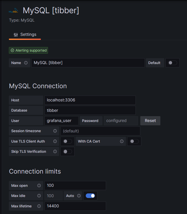
One step where I always stumble again is that in the entry mask for the connection setup, localhost:3306 is proposed in grey color as Host, but unless you type that in, too, Grafana will actually not use localhost:3306. So be sure to physically type that in.
Populating the Database
Tibber customers who have created an API token for themselves [4] can populate the database with the following bash script; in this script, you need to replace _API_TOKEN with your personal API token ( [4]) and _HOME_ID with your personal Home ID ([1]). The script further assumes that the user gabriel can login to the MySQL database without further authentication; this can be achieved by writing the MySQL login information in the file ~/.my.cnf.
#!/bin/bash
#
# Dieses Skript liest Daten für die Tibber-Datenbank und speichert das Ergebnis in einer MySQL-Datenbank ab.
# Das Skript wird einmal pro Tag aufgerufen.
#
# V1.3; 2024-03-24, Gabriel Rüeck <gabriel@rueeck.de>, <gabriel@caipirinha.spdns.org>
#
# CONSTANTS
declare -r    MYSQL_DATABASE='tibber'
declare -r    MYSQL_SERVER='localhost'
declare -r    MYSQL_USER='gabriel'
declare -r    TIBBER_API_TOKEN='_API_TOKEN'
declare -r    TIBBER_API_URL='https://api.tibber.com/v1-beta/gql'
declare -r    TIBBER_HOME_ID='_HOME_ID'

# VARIABLES

# PROGRAM
# Read price information for tomorrow
curl -s -S -H "Authorization: Bearer ${TIBBER_API_TOKEN}" -H "Content-Type: application/json" -X POST -d  '{ "query": "{viewer {home (id: \"'"${TIBBER_HOME_ID}"'\") {currentSubscription {priceInfo {tomorrow {total startsAt level }}}}}}" }' "${TIBBER_API_URL}" | jq -r '.data.viewer.home.currentSubscription.priceInfo.tomorrow[] | .total, .startsAt, .level' | while read cost; do
  read LINE
  read level
  timestamp=$(echo "${LINE%%+*}" | tr 'T' ' ')
  # Determine timezone offset and store the UTC datetime in the database
  offset="${LINE:23}"
  mysql --default-character-set=utf8mb4 -B -N -r -D "${MYSQL_DATABASE}" -h ${MYSQL_SERVER} -u ${MYSQL_USER} -e "INSERT INTO preise (zeitstempel,preis,niveau) VALUES (DATE_SUB(\"${timestamp}\",INTERVAL \"${offset}\" HOUR_MINUTE),${cost},\"${level}\");"
done

# Read consumption information from the past 24 hours
curl -s -S -H "Authorization: Bearer ${TIBBER_API_TOKEN}" -H "Content-Type: application/json" -X POST -d  '{ "query": "{viewer {home (id: \"'"${TIBBER_HOME_ID}"'\") {consumption (resolution: HOURLY, last: 24) {nodes {from to cost consumption}}}}}" }' "${TIBBER_API_URL}" | jq -r '.data.viewer.home.consumption.nodes[] | .from, .consumption, .cost' | while read LINE; do
  read consumption
  read cost
  timestamp=$(echo "${LINE%%+*}" | tr 'T' ' ')
  # Determine timezone offset and store the UTC datetime in the database
  offset="${LINE:23}"
  mysql --default-character-set=utf8mb4 -B -N -r -D "${MYSQL_DATABASE}" -h ${MYSQL_SERVER} -u ${MYSQL_USER} -e "INSERT INTO verbrauch (zeitstempel,energie,kosten) VALUES (DATE_SUB(\"${timestamp}\",INTERVAL \"${offset}\" HOUR_MINUTE),${consumption},${cost});"
done
In my case, I call this script with cron once per day, at 14:45 as Tibber releases the price information for the subsequent day only at 14:00. The script furthermore stores UTC timestamps in the database. Grafana will adjust them to the local time for graphs of the type Time series.
Easy Visualizations
Price level
One of my first visualizations was a table that shows the price level tags for today and tomorrow. The idea behind is that I would look at the table once per day during breakfast and immediately identify the sweet spots on where I could charge the car, turn on the washing machine, etc.
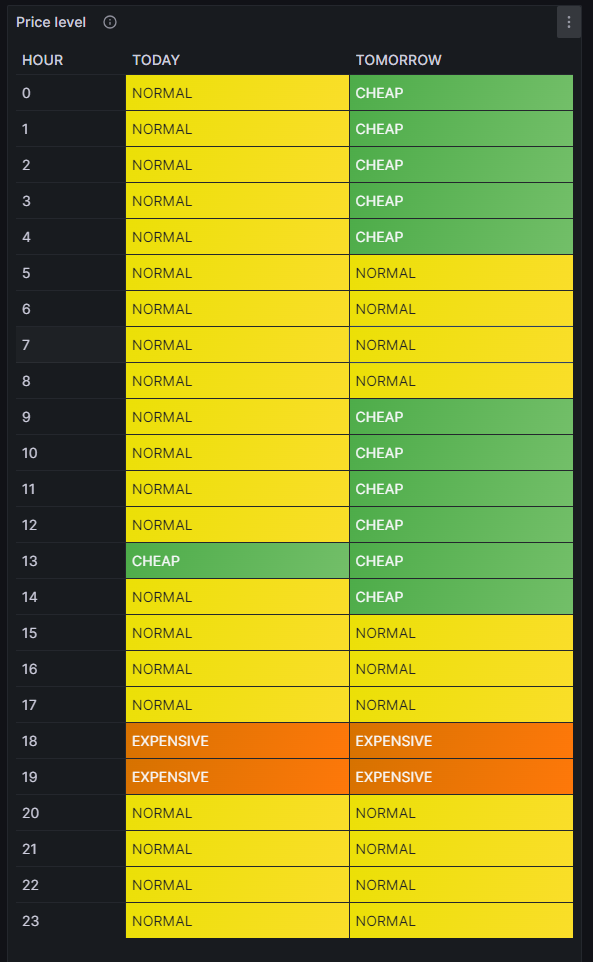
For this table, we use the built-in Grafana visualization Table. We select the according database, and our MySQL query is:
SELECT IF(DATE(DATE_ADD(zeitstempel,INTERVAL HOUR(TIMEDIFF(SYSDATE(),UTC_TIMESTAMP())) HOUR))=CURDATE(),'TODAY','TOMORROW') AS Tag, HOUR(DATE_ADD(zeitstempel,INTERVAL HOUR(TIMEDIFF(SYSDATE(),UTC_TIMESTAMP())) HOUR)) AS Stunde, niveau
FROM preise
WHERE DATE_ADD(zeitstempel,INTERVAL HOUR(TIMEDIFF(SYSDATE(),UTC_TIMESTAMP())) HOUR)>=CURDATE()
Group BY Tag, Stunde;
The query above lists one price level per line. However, in order to get the nice visualization shown above, we need to transpose the table with respect to the months, and therefore, we must select the built-in transformation Grouping to Matrix and enter our column names according to the image below:

Now, in order to get a beautiful visualization, we need to adjust some of the panel options, and those are:
- Cell options → Cell type: Set to Auto
- Standard options → Color scheme: Set to Single color
and we need to define some Value mappings:
- NORMAL → Select yellow color
- EXPENSIVE → Select orange color
- VERY_EXPENSIVE → Select red color
- CHEAP → Select green color
- VERY_CHEAP → Select blue color
and we need to define some Overrides:
- Override 1 → Fields with name: Select TODAY
- Override 1 → Cell options → Cell type: Set to Colored background
- Override 2 → Fields with name: Select TOMORROW
- Override 2 → Cell options → Cell type: Set to Colored background
- Override 3 → Fields with type: Select Stunde\Tag
- Override 3 → Column width → Set to 110
- Override 3 → Standard options → Display name: Type HOUR (That is only necessary because I initially did my query with German column names)
In the MySQL query above, you can find the sequence
DATE_ADD(zeitstempel,INTERVAL HOUR(TIMEDIFF(SYSDATE(),UTC_TIMESTAMP())) HOUR)which actually transforms the UTC timestamp into the timestamp of the local time of the machine where the MySQL server resides. In my case, this is the same machine that I use for Grafana. The sub-sequence
HOUR(TIMEDIFF(SYSDATE(),UTC_TIMESTAMP()))gives – in my case – back a 2 when we are in summer time as then we are at UTC+2h, and 1 when we are in winter time as then we are at UTC+1h. This sequence was necessary for me as the Grafana visualization Table does not do an automatic time conversion to the local time.
Electricity price (per kWh) and grid consumption
In the next visualization, we will look at a timeline of the electricity price per hour and our consumption pattern. This will look like this graph:
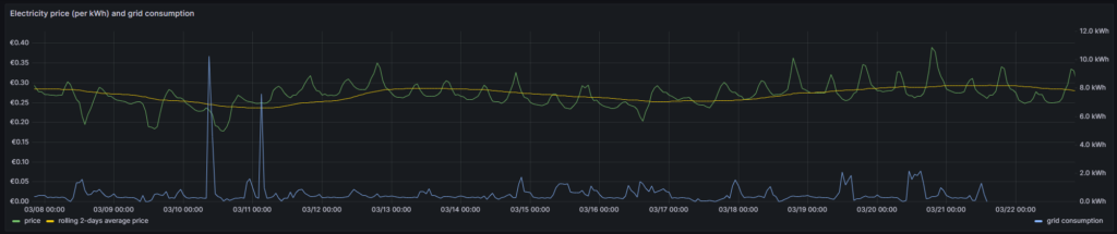
For this graph, we use the built-in Grafana visualization Time series. We select the according database, and we define two MySQL queries. The first one is named Price:
SELECT zeitstempel,
       preis AS 'price',
       AVG(preis) OVER (ORDER BY zeitstempel ROWS BETWEEN 47 PRECEDING AND CURRENT ROW) as 'rolling 2-days average price'
FROM preise;
The first query has the peculiarity that we do not only retrieve the price for each 1-hour block, but that we also calculate a rolling 2-days average over the extracted data. The second query is named Consumption and retrieves our energy consumption:
SELECT zeitstempel, energie AS 'grid consumption' FROM verbrauch;Again, we need to adjust some of the panel options, and those are:
- Standard options → Unit: Select (Euro) €
- Standard options → Min: Set to 0
- Standard options → Decimals: Set to 2
and we need to define some Overrides:
- Override 1 → Fields with name: Select grid consumption
- Override 1 → Axis → Placement: Select Right
- Override 1 → Standard options → Unit: Select Kilowatt-hour (kWh)
- Override 1 → Standard options → Decimals: Set to 1
In this graph, we can already get an indication on how well we time our energy consumption. Ideally, the peaks (local maximums) in energy consumption (blue line) should coincide with the local minimums of the electricity price (green line). As you can see with the two peaks of the blue line (charging the BEV), I did not always match this sweet spot. There might be good reasons for consuming electricity also at hours of higher prices, and some examples are:
- You have to drive away at a certain hour, and you need to charge the BEV now.
- You have solar generation at certain times of the day which you intend to use and therefore consume electricity (like for charging a BEV) when the sun shines. While you then might not consume at the cheapest hour, you might ultimately make good use of the additional solar energy.
- You want to watch TV in the evening when the electricity price is typically high.
This graph visualizes the data according to the timezone of the dashboard, so there is no need to add an offset to the UTC timestamps in the database.
Heatmap of the Tibber flexible hourly prices per kWh
In the next visualization, we look at a heatmap of the hourly prices and therefore, we use the plug-in Grafana visualization Hourly heatmap.
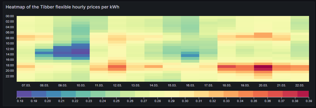
The query is very simple:
SELECT UNIX_TIMESTAMP(DATE_ADD(zeitstempel,INTERVAL HOUR(TIMEDIFF(SYSDATE(),UTC_TIMESTAMP())) HOUR)) AS time, preis FROM preise;However, we need to adjust some of the panel options, and those are:
- Dimensions → Time: Select time
- Dimensions → Value: Select price
- Hourly heatmap → From: Set to 00:00
- Hourly heatmap → To: Set to 00:00
- Hourly heatmap → Group by: Select 60 minutes
- Hourly heatmap → Calculation: Select Sum
- Hourly heatmap → Color palette: Select Spectral
- Hourly heatmap → Invert color palette → Activate
- Legend → Show legend → Activate
- Legend → Gradient quality: Select Low
- Standard options → Unit: Select (Euro) €
- Standard options → Decimals: Set to 2
- Standard options → Color scheme: Select From thresholds (by value)
With the heatmap, we have an easy-to-understand visualization on when the prices are high and on when they are low and on whether there is a regular pattern that we can observe. In this case, we can identify that in the evening (at dinner or TV time), the electricity price often seems to be high. Hence, this is not a good time to switch on powerful electric consumers or to start charging a BEV.
Similar to the Grafana visualization Table, you can find the sequence
DATE_ADD(zeitstempel,INTERVAL HOUR(TIMEDIFF(SYSDATE(),UTC_TIMESTAMP())) HOUR)because the Grafana visualization Hourly heatmap also does not do an automatic time conversion to the local time.
Complex Visualizations
Actual cost versus minimal cost, maximal cost, average cost per day
This visualization shows the daily electricity cost that I have incurred (blue line) and the cost I would have incurred if I had purchased the whole amount of electricity on the respective day:
- … during the cheapest hour on that day (green line)
- … during the most expensive hour on that day (red line)
- … at an average price (average of all hours) on that day (yellow line)
The closer the blue line is to the green line, the better I have shifted my consumption pattern to the hours of cheap electricity. In real life, one will always have to purchase electricity also in hours of expensive electricity unless one switches off all devices in a household at certain hours. So, in real life, the blue line will never be the same as the green line. A blue line between the yellow and the green line already indicates that one does well. The graph also shows that my consumption varies substantially from day to day. The graph uses the built-in Grafana visualization Time series. The last data point must not be considered as the last day is only calculated until 14:00 local time.
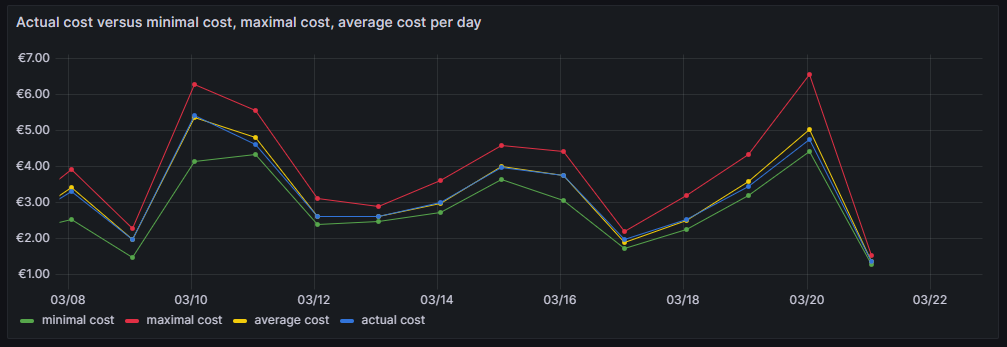
For this graph, we join the tables preise and verbrauch in a MySQL query and group the result by day:
SELECT DATE(preise.zeitstempel) AS 'date',
       MIN(preise.preis)*SUM(verbrauch.energie) AS 'minimal cost',
       MAX(preise.preis)*SUM(verbrauch.energie) AS 'maximal cost',
       AVG(preise.preis)*SUM(verbrauch.energie) AS 'average cost',
       SUM(verbrauch.kosten) AS 'actual cost'
FROM preise JOIN verbrauch ON verbrauch.zeitstempel=preise.zeitstempel
WHERE DATE(preise.zeitstempel)>'2024-03-03'
GROUP BY DATE(preise.zeitstempel);
The following panel options are recommended:
- Standard options → Unit: Select (Euro) €
- Standard options → Decimals: Set to 2
and the following Overrides are recommended:
- Override 1 → Fields with name: Select minimal cost
- Override 1 → Standard options → Color scheme: Select Single color, then select green
- Override 2 → Fields with name: Select maximal cost
- Override 2 → Standard options → Color scheme: Select Single color, then select red
- Override 3 → Fields with name: Select actual cost
- Override 3 → Standard options → Color scheme: Select Single color, then select blue
- Override 4 → Fields with name: Select average cost
- Override 4 → Standard options → Color scheme: Select Single color, then select yellow
Important: This graph adds up the data from a UTC day (not the local calendar day) and visualizes the data points according to the timezone of the dashboard.
Cumulated savings versus various fictive static electricity prices
This visualization shows us in a cumulative manner how much money I have saved using dynamic pricing versus fictive electricity contracts with different static prices per kWh (traditional contracts). The graph uses the built-in Grafana visualization Time series. The last data point must not be considered as the last day is only calculated until 14:00 local time.
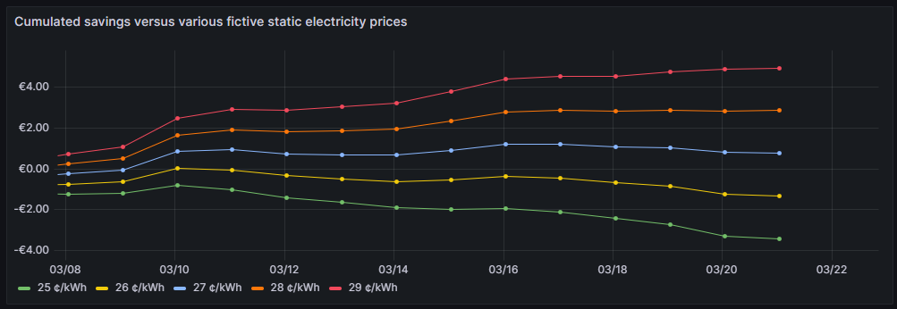
One can see that for traditional prices below 27 ¢/kWh, I would not have saved any money so far. 27 ¢/kWh is the price that I could get in a traditional electricity contract at the place where I live. However, it is too early yet to draw final conclusions. I intend to observe how the graphs advance when we get into summer as I expect that during summer, I will have more times at cheap electricity whereas in the subsequent winter, I will probably have more times at higher prices. The graph is done with this query:
SELECT DATE(preise.zeitstempel) AS 'Datum',
       SUM(0.25*SUM(verbrauch.energie)-SUM(verbrauch.kosten)) OVER (ORDER BY DATE(preise.zeitstempel)) as '25 ¢/kWh',
       SUM(0.26*SUM(verbrauch.energie)-SUM(verbrauch.kosten)) OVER (ORDER BY DATE(preise.zeitstempel)) as '26 ¢/kWh',
       SUM(0.27*SUM(verbrauch.energie)-SUM(verbrauch.kosten)) OVER (ORDER BY DATE(preise.zeitstempel)) as '27 ¢/kWh',
       SUM(0.28*SUM(verbrauch.energie)-SUM(verbrauch.kosten)) OVER (ORDER BY DATE(preise.zeitstempel)) as '28 ¢/kWh',
       SUM(0.29*SUM(verbrauch.energie)-SUM(verbrauch.kosten)) OVER (ORDER BY DATE(preise.zeitstempel)) as '29 ¢/kWh'
FROM preise JOIN verbrauch ON verbrauch.zeitstempel=preise.zeitstempel
WHERE DATE(preise.zeitstempel)>'2024-03-03'
GROUP BY DATE(preise.zeitstempel);
The following panel options are recommended:
- Standard options → Unit: Select (Euro) €
- Standard options → Decimals: Set to 2
Important: This graph adds up the data from a UTC day (not the local calendar day) and visualizes the data points according to the timezone of the dashboard.
Daily savings using Tibber flexible versus a fictive static price of 27 ¢/kWh
This next visualization shows how much money I have saved (green) or lost (red) using dynamic pricing versus a fictive electricity contract with a price of 27 ¢/kWh that – as mentioned before – I could get in a traditional electricity contract at the place where I live. The graph uses the built-in Grafana visualization Bar chart. The last data point must not be considered as the last day is only calculated until 14:00 local time.
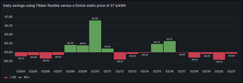
One can see that due to the nature of dynamic prices, I do not save money every day. It has been quite a mixed result so far. The graph is done with this query:
SELECT DATE_FORMAT(preise.zeitstempel,'%m/%d') AS 'Datum',
       0.27*SUM(verbrauch.energie)-SUM(verbrauch.kosten) AS 'Daily cost vs. average'
FROM preise JOIN verbrauch ON verbrauch.zeitstempel=preise.zeitstempel
WHERE DATE(preise.zeitstempel)>'2024-03-03'
GROUP BY DATE(preise.zeitstempel);
The following panel options are recommended:
- Bar chart → Color by field: Select Daily cost vs. average
- Standard options → Unit: Select (Euro) €
- Standard options → Decimals: Set to 2
- Standard options → Color scheme: Select From thresholds (by value)
- Thresholds → Enter 0, then select green
- Thresholds → Base: Select red
Important: This graph adds up the data from a UTC day (not the local calendar day).
Daily savings using Tibber flexible versus Tibber daily average price
A similar visualization shows how much money I have saved (green) or lost (red) using dynamic pricing versus the average price per day, calculated on all dynamic prices of that day. This graph shows me if I am successful in making use of dynamic pricing (green) or not (red). The graph uses the built-in Grafana visualization Bar chart. The last data point must not be considered as the last day is only calculated until 14:00 local time.
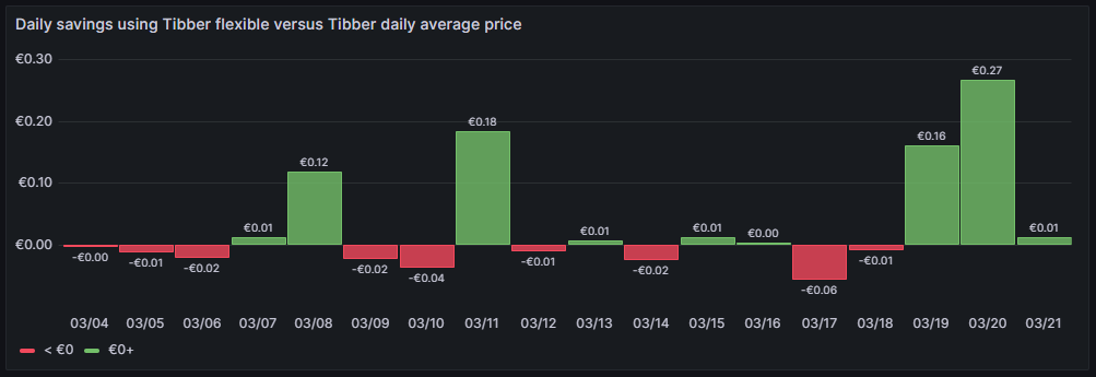
So far, it seems that while I do have “good” and “bad” days, on on the good days, I seem to save more money compared to the Tibber average price. The large green bars are those where I charge the BEV, and before I charge the BEV, I really carefully consider the electricity price of today and tomorrow. This graph is done with this query:
SELECT DATE_FORMAT(preise.zeitstempel,'%m/%d') AS 'Datum',
       AVG(preise.preis)*SUM(verbrauch.energie)-SUM(verbrauch.kosten) AS 'Daily cost vs. average'
FROM preise JOIN verbrauch ON verbrauch.zeitstempel=preise.zeitstempel
WHERE DATE(preise.zeitstempel)>'2024-03-03'
GROUP BY DATE(preise.zeitstempel);
The following panel options are recommended:
- Bar chart → Color by field: Select Daily cost vs. average
- Standard options → Unit: Select (Euro) €
- Standard options → Decimals: Set to 2
- Standard options → Color scheme: Select From thresholds (by value)
- Thresholds → Enter 0, then select green
- Thresholds → Base: Select red
Important: This graph adds up the data from a UTC day (not the local calendar day).
Cost of purchased electricity from grid with price indication
This is one of my favorite graphs as it contains a lot of information in one visualization. It shows the electricity cost per day, but also, how this cost is composed. Each day is a concatenation of 24 rectangles. The 24 rectangles represent the 24 hours of the day. Their color is different, ranging in shades from green to red. The green only rectangle (rgb: 0, 255, 0) is the cost that incurred at the cheapest hour of the day. The red only rectangle (rgb: 255, 0, 0) is the cost that incurred at the most expensive hour of the day. The shades in between ranging from green to red represent an ordered list of the hours from cheap to expensive. Large rectangles mean that a large part of the daily cost can be attributed to a consumption in that hour. Essentially, this means that the more green shades a day has, the more cost has incurred at hours of cheap electricity and the better I have used the dynamic pricing for me. The more red shades a day has, the more cost has incurred at hours of expensive electricity. A day with more red shades is not automatically a “bad” day. There might be reasons for a consumption at expensive hours, and some which are true in my case, are:
- I might cover the electricity demand at cheap hours by my solar panels so that during these hours, I do not have any grid consumption at all.
- I might deliberately decide to consume electricity at expensive hours during daylight because my solar panels cover a large part of the consumption at my home, maybe, because I charge the car and 50% of the electric energy comes from the solar panels anyway and I just buy the remaining 50% from the grid. While the grid consumption might be expensive, I anyway get 50% “for free” from the solar panels.
- I might deliberately decide to consume electricity at expensive hours because the ambient temperature outside the house is moderate or warm and I can heat the house with the air conditioner at high efficiency while I can switch off the central heating which runs by natural gas. In that case, even at high prices, I expect to have a better outcome overall because I might be able to switch off the central heating completely.
The graph uses the built-in Grafana visualization Bar chart. The last data point must not be considered as the last day is only calculated until 14:00 local time.
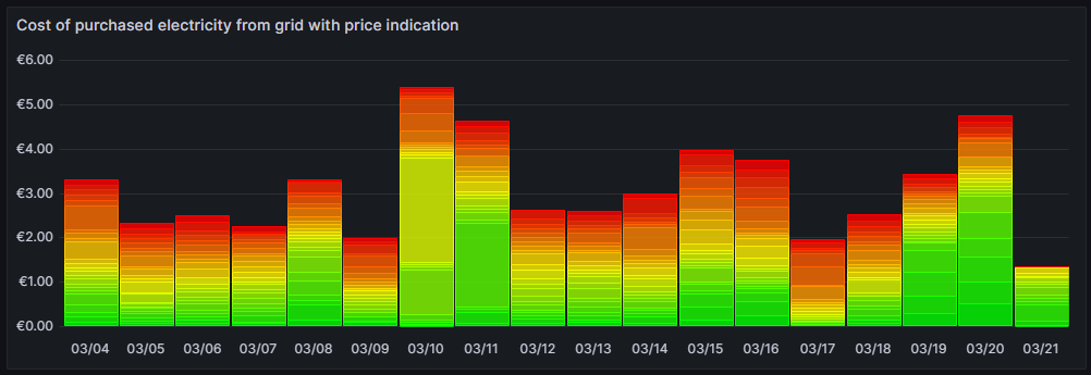
This graph uses this query:
SELECT DATE_FORMAT(preise.zeitstempel,'%m/%d') AS 'Datum',
       ROW_NUMBER() OVER (PARTITION BY DATE(preise.zeitstempel) ORDER BY preise.preis ASC) AS 'Row',
	   verbrauch.kosten AS 'Kosten'
FROM preise JOIN verbrauch ON verbrauch.zeitstempel=preise.zeitstempel
WHERE DATE(preise.zeitstempel)>'2024-03-03'
ORDER BY DATE(preise.zeitstempel) ASC, preise.preis ASC;
and the built-in transformation Grouping to Matrix:

The following panel options must be used:
- Standard options → Unit: Select (Euro) €
- Standard options → Min: Set to 0
- Standard options → Decimals: Set to 2
Additionally, we need to define exactly 24 Overrides:
- Override 1 → Fields with name: Select 1
- Override 1 → Standard options → Color scheme: Select Single color, then select Custom, then rgb(0, 255, 0)
- Override 2 → Fields with name: Select 2
- Override 2 → Standard options → Color scheme: Select Single color, then select Custom, then rgb(22, 255, 0)
- Override 3 → Fields with name: Select 3
- Override 3 → Standard options → Color scheme: Select Single color, then select Custom, then rgb(44, 255, 0)
- Override 4 → Fields with name: Select 4
- Override 4 → Standard options → Color scheme: Select Single color, then select Custom, then rgb(66, 255, 0)
- Override 5 → Fields with name: Select 5
- Override 5 → Standard options → Color scheme: Select Single color, then select Custom, then rgb(89, 255, 0)
- Override 6 → Fields with name: Select 6
- Override 6 → Standard options → Color scheme: Select Single color, then select Custom, then rgb(111, 255, 0)
- Override 7 → Fields with name: Select 7
- Override 7 → Standard options → Color scheme: Select Single color, then select Custom, then rgb(133, 255, 0)
- Override 8 → Fields with name: Select 8
- Override 8 → Standard options → Color scheme: Select Single color, then select Custom, then rgb(155, 255, 0)
- Override 9 → Fields with name: Select 9
- Override 9 → Standard options → Color scheme: Select Single color, then select Custom, then rgb(177, 255, 0)
- Override 10 → Fields with name: Select 10
- Override 10 → Standard options → Color scheme: Select Single color, then select Custom, then rgb(199, 255, 0)
- Override 11 → Fields with name: Select 11
- Override 11 → Standard options → Color scheme: Select Single color, then select Custom, then rgb(222, 255, 0)
- Override 12 → Fields with name: Select 12
- Override 12 → Standard options → Color scheme: Select Single color, then select Custom, then rgb(244, 255, 0)
- Override 13 → Fields with name: Select 13
- Override 13 → Standard options → Color scheme: Select Single color, then select Custom, then rgb(255, 244, 0)
- Override 14 → Fields with name: Select 14
- Override 14 → Standard options → Color scheme: Select Single color, then select Custom, then rgb(255, 222, 0)
- Override 15 → Fields with name: Select 15
- Override 15 → Standard options → Color scheme: Select Single color, then select Custom, then rgb(255, 200, 0)
- Override 16 → Fields with name: Select 16
- Override 16 → Standard options → Color scheme: Select Single color, then select Custom, then rgb(255, 177, 0)
- Override 17 → Fields with name: Select 17
- Override 17 → Standard options → Color scheme: Select Single color, then select Custom, then rgb(255, 155, 0)
- Override 18 → Fields with name: Select 18
- Override 18 → Standard options → Color scheme: Select Single color, then select Custom, then rgb(255, 133, 0)
- Override 19 → Fields with name: Select 19
- Override 19 → Standard options → Color scheme: Select Single color, then select Custom, then rgb(255, 110, 0)
- Override 20 → Fields with name: Select 20
- Override 20 → Standard options → Color scheme: Select Single color, then select Custom, then rgb(255, 89, 0)
- Override 21 → Fields with name: Select 21
- Override 21 → Standard options → Color scheme: Select Single color, then select Custom, then rgb(255, 66, 0)
- Override 22 → Fields with name: Select 22
- Override 22 → Standard options → Color scheme: Select Single color, then select Custom, then rgb(255, 44, 0)
- Override 23 → Fields with name: Select 23
- Override 23 → Standard options → Color scheme: Select Single color, then select Custom, then rgb(255, 22, 0)
- Override 24 → Fields with name: Select 24
- Override 24 → Standard options → Color scheme: Select Single color, then select Custom, then rgb(255, 0, 0)
Important: This graph adds up the data from a UTC day (not the local calendar day).
Conclusion
Even with a relatively simple dataset, we can create insightful visualizations with Grafana that can help us to interpret complex relationships. In my case, the visualizations shall help me to answer the questions:
- Do I fare well with dynamic pricing as compared to a traditional electricity contract with static prices?
- Am I able to shift consumption pattern of large energy chunks efficiently to those hours where electricity is cheaper?
As I mentioned, there might be reasons to buy electricity also at expensive hours. The fact that I have support of solar panels during the day might tilt the decision to consume electric energy aways from the cheapest hours to hours where a large part of that consumption is anyway covered by the solar panels. Or I might decide to heat with the air conditioners because the temperature difference between outside and inside of the house is small and the air conditioners can run with a high efficiency. In that case, I trade in natural gas consumption versus electricity consumption.
Outlook
It would be interesting to consider the energy that the solar panels generate “for free” (not really for free, but as they have been installed, they are already “sunk cost”) and visualize the resulting electricity cost from the mix of solar energy with energy consumed from the grid.
Likewise, it might be interesting as well as challenging to derive a good model that uses a battery and dynamic electricity prices as well as the energy from the solar panels to minimize cost of the energy consumption from the grid. How large should this battery be? When should it be charged from the grid and when should it return its energy to the consumers in the house?
Files
The following dataset was used for the graphs:
Sources
- [1] = Tibber Developer
- [2] = Download Grafana | Grafana Labs
- [3] = day-ahead market – an overview
- [4] = Tibber Developer: Communicating with the API
Disclaimer
- Program codes and examples are for demonstration purposes only.
- Program codes are not recommended be used in production environments without further enhancements in terms of speed, failure-tolerance or cyber-security.
- While program codes have been tested, they might still contain errors.
- I am in neither affiliated nor linked to companies named in this blog post.
Getting around Carrier-grade NAT
Executive Summary
This blog post explains how a small internet-based shared server (“vServer”, “VPS”) can be used to tunnel connections from the internet back to a SoHo-based router that does not have a publicly routable IPv4 internet address, maybe because the internet service provider (ISP) uses Carrier-grade NAT (CG-NAT) and only offers “real” IPv4 addresses at cost. As internet-based shared servers can be rented for small fees, the approach described below is a viable concept to overcome the limitations of CG-NAT connections which might only allow outgoing connections for IPv4 or even for both IPv4 and IPv6. This concept can even be used if the SoHo server is connected via the mobile network to the internet-based shared server.
Background
The implementation proved useful for me when I switched from my DSL ISP who happily had provided me with “real” (routable) IPv4 and IPv6 addresses to a new fiber-optics ISP that provides IPv6, but that uses CG-NAT on IPv4 so that no incoming IPv4 connections are possible from the internet. As I feared that my server at home would only be accessible from the internet via IPv6, I had to develop this counterstrategy.
Preconditions
In order to use the approach described here, you should:
- … have access to a Linux machine which is already properly configured for dual stack on its principal network interface (e.g., eth0)
- … additionally have access to a cloud-based Linux server which is already properly configured for dual stack on its principal network interface
- … have access to a DNS resolver where you can enter an IPv4 and an IPv6 addresses for your SoHo server so that your domain resolves properly
- … have the package openvpn installed on both machines (preferably from a repository of your Linux distribution)
- … know how to create client and server certificates for openvpn [1]
- … have knowledge of routing concepts, networks, some understanding of shell scripts and configuration files
- … know related system commands like sysctl
- … familiarize yourself with [2], [3], [4], [5]
Description and Usage
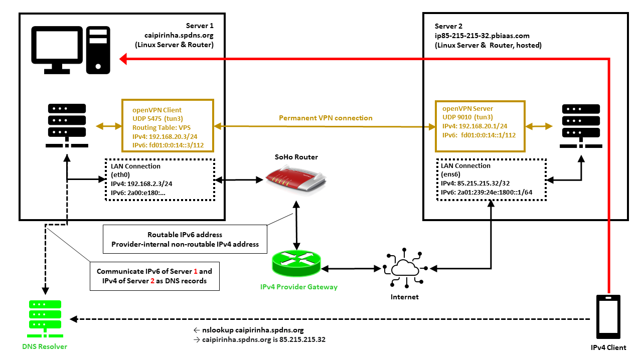
In this setup, we have a full-blown SoHo server (Server 1) which is hosting numerous services that we want to offer to the world. However, while the provider allocates an IPv6 /64 subnet, he does not offer an IPv4 address that would be reachable from the internet. Rather than that, he employs Carrier-grade NAT (CG-NAT) for IPv4. This is a typical setup for fiber-optics or cable providers or for mobile network providers. In some countries (which came late to the internet), IPv4 addresses are scarce in general, and so you might experience CG-NAT for all private internet connections.
This is where Server 2 comes into play. Server 2 is a hosted shared server, it just needs a good internet connection and a fixed IPv4 address, but it does not need a lot of computational power. It will only be used to forward traffic to Server 1. In my case, I rented a small “VPS” server from Ionos as I personally found their offer compelling [6], but there are alternatives. My VPS has a dual-stack and a fixed IPv4 address and a fixed IPv6 /64 subnet allocated. The IPv4 address of the VPS is 85.215.215.32, and we will use this IPv4 address as entry address for our SoHo server (Server 1) caipirinha.spdns.org.
A new Routing Table
We want to separate the traffic that we receive and send out in return via the VPN network (192.168.20.0/24) from the regular traffic that enters and leaves the server via the network 192.168.2.0/24. Therefore, we set up a new routing table as described in [7] and name it “VPS”. In order to access it via its name, we modify /etc/iproute2/rt_tables:
#
# reserved values
#
255 local
254 main
253 default
0 unspec
#
# local
#
#1  inr.ruhep

...
201 VPS
...
Setting up a permanent VPN
First, we need to set up a permanent VPN connection from Server 1 to Server 2. Server 1 will be the VPN client, and Server 2 will be the VPN server. I chose this direction because in that approach, Server 1 may even be connected to the internet via a mobile only connection CG-NAT both on IPv4 and IPv6. In my approach, I use the network 192.168.20.0/24 for the VPN connection; Server 1 gets the address 192.168.20.3 and Server 2 gets the address 192.168.20.1.
Server 2: The VPN Server
On Server 2, we set up a VPN server listening on port 9010 (UDP), using dev tun3. The configuration file is shown below. In my case, Server 2 is an Ubuntu-based server, and so it is recommended to adjust the settings in the configuration file /etc/default/openvpn which governs the behavior of openvpn connections on Ubuntu. I modified this configuration file so that only one openvpn service is started. This is done via the configuration option
AUTOSTART="server-9010"For the configuration of the server side, I meanwhile include the CA certificate, the server certificate and the private key in one configuration file. I find that more convenient, but it certainly may have disadvantages, The key message is that it is possible to do so. My own certificates and private keys have been substituted by “…” here, of course.
# Konfigurationsdatei für den openVPN-Server auf IONOS VPS (UDP:9010)

client-config-dir     /etc/openvpn/server/conf-9010
crl-verify            /etc/openvpn/server/crl.pem
dev                   tun3
dh                    /etc/openvpn/server/dh.pem
hand-window           90
ifconfig              192.168.20.1  255.255.255.0
ifconfig-pool         192.168.20.2  192.168.20.254  255.255.255.0
ifconfig-ipv6         fd01:0:0:14::1 2a01:239:24e:1800::1
ifconfig-ipv6-pool    fd01:0:0:14::2/112
ifconfig-pool-persist /etc/openvpn/server/ip-pool-9010.txt
keepalive             20 80
log                   /var/log/openvpn/server-9010.log
mode                  server
persist-key
persist-tun
port                  9010
proto                 udp6
reneg-sec             86400
script-security       2
status                /var/run/openvpn/status-9010
tls-server
topology              subnet
verb                  1
writepid              /var/run/openvpn/server-9010.pid

# Topologie des VPN und Default-Gateway
push "topology subnet"
push "tun-ipv6"

<ca>
-----BEGIN CERTIFICATE-----
...
-----END CERTIFICATE-----
</ca>

<cert>
-----BEGIN CERTIFICATE-----
...
-----END CERTIFICATE-----
</cert>

<key>
-----BEGIN PRIVATE KEY-----
...
-----END PRIVATE KEY-----
</key>
We also must take care that our client always gets the IP address 192.168.20.3 as we originally envisioned. This is done with the client-specific configuration file /etc/openvpn/server/conf-9010/caipirinha_client:
# Spezielle Konfigurationsdatei für den Server caipirinha.spdns.org als Client
#

ifconfig-push      192.168.20.3 255.255.255.0
ifconfig-ipv6-push fd01:0:0:14::3/111 fd01:0:0:14::1
The client-specific configuration file additionally also allocates the static IPv6 address fd01:0:0:14::3 to our client. Finally, the service can then be started with:
systemctl start openvpn@server-9010.serviceServer 1: The VPN Client
On Server 1, we set up a VPN client using dev tun3. The local port shall always be 5475 (arbitrarily chosen but fixed so that we can track the connection easily if necessary). Server 2 is addressed via its public IPv6 address (2a01:239:24e:1800::1), but we could also have used its public IPv4 address (85.215.215.32). I chose the IPv6 address because the IPv4 connection would run via the provider gateway, and that might slow down the connection or make it less reliable.
# Konfigurationsdatei für den openVPN-Client auf caipirinha.spdns.org zum IONOS-Server

client
dev              tun3
explicit-exit-notify
hand-window      90
keepalive        10 60
log              /var/log/openvpn_ionos_vpn.log
lport            5475
persist-key
persist-tun
proto            udp
remote           2a01:239:24e:1800::1 9010
remote-cert-tls  server
remote-random
reneg-sec        86400
route-nopull
script-security  2
status           /var/run/openvpn/status_ionos_vpn
up               /etc/openvpn/start_piavpn.sh
verb             1

<ca>
-----BEGIN CERTIFICATE-----
...
-----END CERTIFICATE-----
</ca>

<cert>
-----BEGIN CERTIFICATE-----
...
-----END CERTIFICATE-----
</cert>

<key>
-----BEGIN PRIVATE KEY-----
...
-----END PRIVATE KEY-----
</key>
One peculiarity is the referenced script /etc/openvpn/start_piavpn.sh. At the start of the VPN connection, this script populates the routing table VPS:
#!/bin/bash
#
# This script requires the tool "ipcalc" which needs to be installed on the target system.

# Set the correct PATH environment
PATH='/sbin:/usr/sbin:/bin:/usr/bin'

VPN_DEV=$1
VPN_SRC=$4
VPN_MSK=$5

VPN_GW=$(ipcalc ${VPN_SRC}/${VPN_MSK} | sed -n 's/^HostMin:\s*\([0-9]\{1,3\}\.[0-9]\{1,3\}\.[0-9]\{1,3\}\.[0-9]\{1,3\}\).*/\1/p')
VPN_NET=$(ipcalc ${VPN_SRC}/${VPN_MSK} | sed -n 's/^Network:\s*\([0-9]\{1,3\}\.[0-9]\{1,3\}\.[0-9]\{1,3\}\.[0-9]\{1,3\}\/[0-9]\{1,2\}\).*/\1/p')

case "${VPN_DEV}" in
  "tun0") ROUTING_TABLE='Portugal';;
  "tun1") ROUTING_TABLE='Brasilien';;
  "tun2") ROUTING_TABLE='Singapur';;
  "tun3") ROUTING_TABLE='VPS';;
  "tun8") ROUTING_TABLE='China';;
esac

...

ip route add ${VPN_NET} dev ${VPN_DEV} proto static scope link src ${VPN_SRC} table ${ROUTING_TABLE}
ip route replace default dev ${VPN_DEV} via ${VPN_GW} table ${ROUTING_TABLE}
When the VPN connection is stopped, then the VPN network and the default route are automatically deleted from the routing table VPS as the VPN network collapses. While the VPN connection is up, we can view the routing table VPS with:
caipirinha:~ # ip route list table VPS
default via 192.168.20.1 dev tun3
192.168.20.0/24 dev tun3 proto static scope link src 192.168.20.3
Finally, the client can be started with:
systemctl start openvpn@client_ionos_vps.serviceOf course, the actual name after “openvpn@” in this command depends on how you named the respective client configuration file.
Channeling the Traffic
Now, we must make sure that traffic that is received by Server 2 and that shall be forwarded to Server 1 is channeled in an appropriate way through the VPN connection. We need to execute some commands on both servers. [3], [4] explain how that can be achieved.
Server 2: Forward the traffic
We need to enable IPv4 routing and simply forward connections to those ports where we offer our service on Server 1. This is done by:
sysctl -w net.ipv4.ip_forward=1

iptables -t nat -A PREROUTING -p tcp -m multiport --dports 20,21,25,80,443,465,587,873,993,3000,4078:4088,8009,8080:8082 -j DNAT --to-destination 192.168.20.3
iptables -t nat -A PREROUTING -p udp -m multiport --dports 1194,2372:2380,4396,44576 -j DNAT --to-destination 192.168.20.3
We need two iptables commands, one for TCP connections and one for UDP connections. Both are located in the PREROUTING chain. As we can see, we can combine various ports and even port ranges that shall be forwarded in one command, that is very handy. Of course, you should only forward the ports that correspond to services on Server 1 that you want to offer to the world. It is also possible to offer the services on different ports on Server 2, so that http is listening on port 81 TCP rather than on 80 TCP although in my opinion, that does not make much sense.
Let us assume that a client initiates a connection to Server 2 on port 80 (http). The first iptables command changes the destination IP from the IP address of Server 2 (85.215.215.32) to the IP address 192.168.20.3 which is the VPN client on Server 1. As we have enabled routing on Server 2, the packet is routed from ens6 to tun3 and leaves Server 2 via the VPN connection to Server 1.
Server 1: Accept the traffic in Routing Table VPS
Server 1 receives the traffic and needs to channel it via routing table VPS. This is done with the command:
ip rule add from 192.168.20.3 priority 1000 table VPSThe beauty of this command is that the outgoing traffic will also use table VPS and therefore leave Server 1 not via the default interface eth0 to the SoHo router, but via tun3 back to Server 2 (see [4], [8]). We can identify the traffic that we receive from Server 2 at Server 1 with the conntrack command:
caipirinha:~ # conntrack -L | fgrep "192.168.20"
tcp      6 117 TIME_WAIT src=109.250.125.241 dst=192.168.20.3 sport=55370 dport=80 src=192.168.20.3 dst=109.250.125.241 sport=80 dport=55370 [ASSURED] mark=0 use=1
tcp      6 117 TIME_WAIT src=109.250.125.241 dst=192.168.20.3 sport=55366 dport=80 src=192.168.20.3 dst=109.250.125.241 sport=80 dport=55366 [ASSURED] mark=0 use=1
tcp      6 117 TIME_WAIT src=109.250.125.241 dst=192.168.20.3 sport=55368 dport=80 src=192.168.20.3 dst=109.250.125.241 sport=80 dport=55368 [ASSURED] mark=0 use=1
In that case, we have observed a https request (dport=80) from the source IP 109.250.125.241 which has been tunneled via our VPN from Server 2 to Server 1. The client (represented by a mobile phone in the image above) has basically access Server 2 along the red arrow drawn in the image. The benefit of the concept described here is also that the source address (here: 109.250.125.241) is not concealed and therefore, filtering can be done on Server 1 with iptables as if Server 1 was accessed directly. Furthermore, the correct client IP address is in the respective log files.
Other approaches which use SNAT on Server 2 would conceal the source address of the client and therefore, such filtering would have to occur on Server 2 already. The logs on Server 1 however would contain 192.168.20.1 as sole source address for all incoming connections which is why such an approach is not suitable.
Updating the DNS Server
Now we should spend some thoughts on the domain name resolution of Server 1. In my case, I already had a script that communicated any change of the IP address of Server 1 provoked by the ISP almost on a daily basis to a Dynamic DNS (DDNS) provider which so far has done the name resolution for clients that want to access Server 1. I use my own script, but most DDNS providers also offer pre-written scripts for certain architectures or routers.
In our concept though, we must communicate the IPv6 address of Server 1 and the IPv4 address of Server 2 to our DDNS service. As Server 2 has a static IPv4 address, adapting any script should be easy. Alternatively, one could limit the script to only update the IPv6 address of Server 1 and enter the static IPv4 address via the web-based user interface of the DDNS hoster.
Conclusion
This blog post shows how we can channel back traffic via a small internet-based server to a powerful server that is connected via CG-NAT and that may therefore not be accessible directly from the internet. With the approach described here, Server 1 can even be located in a mobile network or inside a firewalled environment as long as the firewall permits outgoing openvpn connections.
Sources
- [1] = Setting up your own Certificate Authority (CA) and generating certificates and keys for an OpenVPN server and multiple clients
- [2] = Setting up Dual Stack VPNs
- [3] = iptables – Port forwarding over OpenVpn
- [4] = Routing for multiple uplinks/providers
- [5] = Predictable Network Interface Names
- [6] = vServer Günstig Mieten » VPS ab 1€ / M.
- [7] = Setting up Client VPNs, Policy Routing
- [8] = Two Default Gateways on One System
Grafana Visualizations (Part 1)
Executive Summary
In this article, we do first steps into visualizations in Grafana of data stored in a MariaDB database and draw conclusions from the visualizations. In this case, we look at meaningful data from solar power generation.
Preconditions
In order to use the approach described here, you should:
- … have access to a Linux machine or account
- … have a MySQL or MariaDB database server installed, configured, up and running
- … have a populated MySQL or MariaDB database like in our example to which you have access
- … have the package Grafana [2] installed, configured, up and running
- … have some basic knowledge of how to operate in a Linux environment and some basic understanding of shell scripts
Description and Usage
The base for the following visualizations is a fully populated database of the following structure:
# Datenbank für Analysen der Solaranlage
# V1.1; 2023-12-10, Gabriel Rüeck <gabriel@rueeck.de>, <gabriel@caipirinha.spdns.org>
# Delete existing databases
REVOKE ALL ON solaranlage.* FROM 'gabriel';
DROP DATABASE solaranlage;

# Create a new database
CREATE DATABASE solaranlage DEFAULT CHARSET utf8mb4 COLLATE utf8mb4_general_ci;
GRANT ALL ON solaranlage.* TO 'gabriel';
USE solaranlage;
SET default_storage_engine=Aria;

CREATE TABLE anlage          (uid            INT UNSIGNED NOT NULL PRIMARY KEY AUTO_INCREMENT,\
                              zeitstempel    TIMESTAMP NOT NULL DEFAULT CURRENT_TIMESTAMP,\
                              leistung       INT UNSIGNED DEFAULT NULL,\
energie INT UNSIGNED DEFAULT NULL);[1] explains how such a database can be filled with real-world data using smart home devices whose data is then stored in the database. For now, we assume that the database already is fully populated and contains large amount of data of the type:
MariaDB [solaranlage]> SELECT * FROM anlage LIMIT 20;
+-----+---------------------+----------+---------+
| uid | zeitstempel         | leistung | energie |
+-----+---------------------+----------+---------+
|   1 | 2023-05-02 05:00:08 |        0 | 5086300 |
|   2 | 2023-05-02 05:15:07 |        0 | 5086300 |
|   3 | 2023-05-02 05:30:07 |        0 | 5086300 |
|   4 | 2023-05-02 05:45:07 |        0 | 5086300 |
|   5 | 2023-05-02 06:00:07 |        0 | 5086300 |
|   6 | 2023-05-02 06:15:07 |    12660 | 5086301 |
|   7 | 2023-05-02 06:30:07 |    39830 | 5086307 |
|   8 | 2023-05-02 06:45:08 |    44270 | 5086318 |
|   9 | 2023-05-02 07:00:07 |    78170 | 5086333 |
|  10 | 2023-05-02 07:15:07 |   187030 | 5086367 |
|  11 | 2023-05-02 07:30:07 |   312630 | 5086424 |
|  12 | 2023-05-02 07:45:08 |   665900 | 5086556 |
|  13 | 2023-05-02 08:00:07 |   729560 | 5086733 |
|  14 | 2023-05-02 08:15:08 |   573700 | 5086889 |
|  15 | 2023-05-02 08:30:07 |   288030 | 5086985 |
|  16 | 2023-05-02 08:45:07 |   444170 | 5087065 |
|  17 | 2023-05-02 09:00:08 |   655880 | 5087217 |
|  18 | 2023-05-02 09:15:07 |   974600 | 5087476 |
|  19 | 2023-05-02 09:30:08 |  1219150 | 5087839 |
|  20 | 2023-05-02 09:45:07 |   772690 | 5088024 |
+-----+---------------------+----------+---------+
20 rows in set (0,000 sec)
whereby the values in column leistung represent the current power generation in mW and the values in energy represent the accumulated energy in Wh.
Now we shall visualize the data of the solar power generation in Grafana. Grafana is powerful and mighty visualization tool with which you can create state-of-the-art dashboards and professional visualizations. I must really laude the team behind Grafana for making such a powerful tool free for personal and other usage (for details to their licenses und usage models, see Licensing | Grafana Labs).
Before you can use data from a MySQL database in Grafana, you have to set up MySQL as a data source in Connections. Remember that MySQL is one of many possible data sources for Grafana and so, you have to walk through the jungle of offered data sources and find the MySQL connection and set up your data source accordingly. On my server, both Grafana and MariaDB run on the same machine, so there is no need for encryption, etc. My setup simply looks like this:
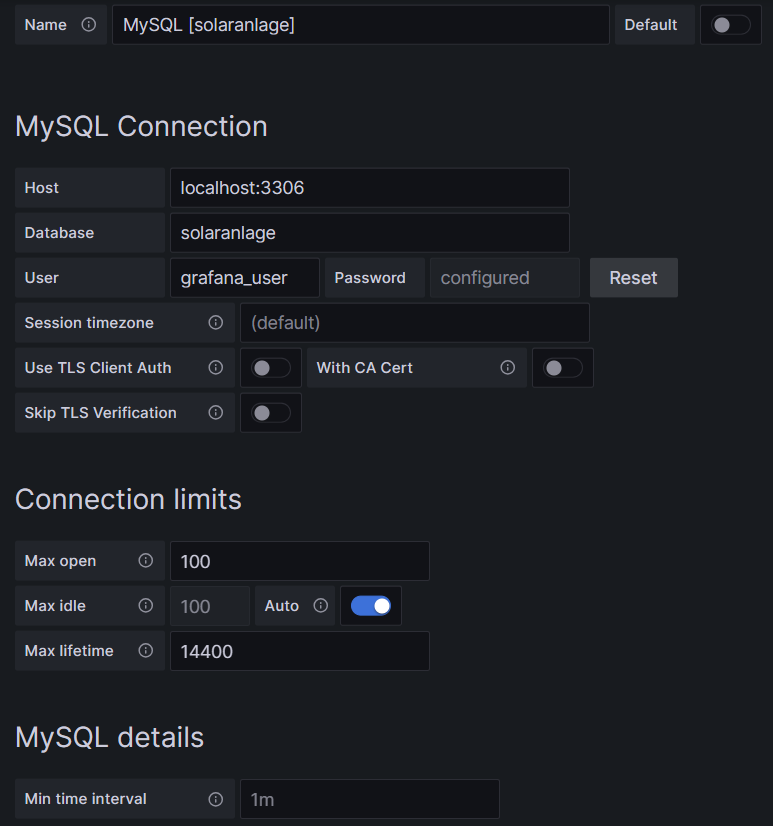
One step where I always stumble again is that in the entry mask for the connection setup, localhost:3306 is proposed in grey color as Host, but unless you type that in, too, Grafana will actually not use localhost:3306. So be sure to physically type that in.
Average Power per Month and Hour of the Day (I)
For this, we use the built-in Grafana visualization Table. We select the according database, and our MySQL query is:
SELECT MONTHNAME(zeitstempel) AS Monat, HOUR(zeitstempel) AS Stunde, ROUND(AVG(leistung)/1000) AS Leistung
FROM anlage
GROUP BY Monat, Stunde
ORDER BY FIELD (Monat,'January','February','March','April','May','June','July','August','September','October','November','December'), Stunde ASC;
This query delivers us an ordered list of power values grouped and ordered by (the correct sequence of) month, and subsequently by the hour of the day as shown below:
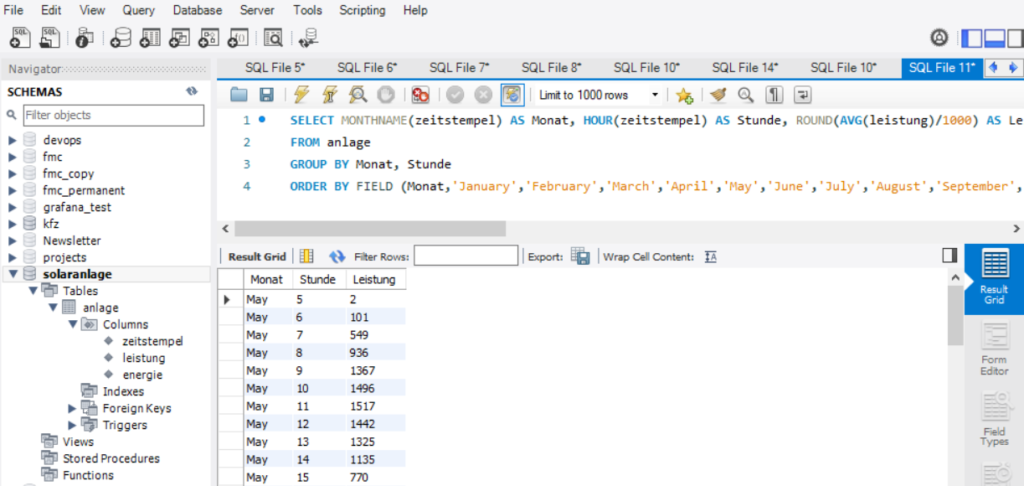
However, this is not enough to get the table view we want in Grafana as the power values are still one-dimensional (only one value per line). We need to transpose the table with respect to the months, and therefore, we must select the built-in transformation Grouping to Matrix for this visualization and enter our column names according to the image below:
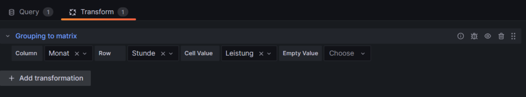
Now, in order to get a beautiful visualization, we need to adjust some of the panel options, and those are:
- Cell options → Cell type: Set to Colored background
- Standard options → Color scheme: Set to Green-Yellow-Red (by value)
and we need to define some Overrides:
- Override 1 → Fields with name: Select Stunde\Monat
- Override 1 → Cell options → Cell type: Set to Auto
- Override 2 → Fields with type: Select Number
- Override 2 → Standard options → Unit: Select Watt (W)
Then, ideally, you should see something like this:
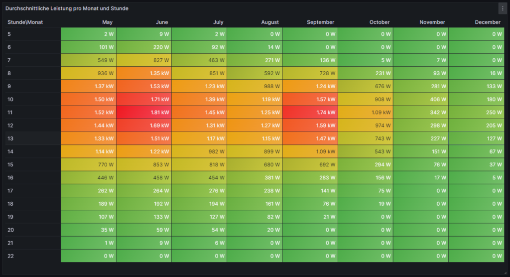
Average Power per Month and Hour of the Day (II)
This visualization is similar to the one of the previous chapter. However, we slightly modify the MySQL query to:
SELECT MONTHNAME(zeitstempel) AS Monat, HOUR(zeitstempel) AS Stunde, ROUND(GREATEST((AVG(leistung)-STDDEV(leistung))/1000,0.0)) AS 'Ø-1σ'
FROM anlage
GROUP BY Monat, Stunde
ORDER BY FIELD (Monat,'January','February','March','April','May','June','July','August','September','October','November','December'), Stunde ASC;
Doing so, we assume that there is some reasonable normal distribution in the timeframe of one month among the values in the same hourly time interval which, strictly speaking, is not true. Further below, we will look into this assumption. Using this unproven assumption, if we subtract 1σ from the average power value and use the resulting value or zero (whichever is higher), then we come to a value where we can say: “Probably (84%), in this month and in this hour, we generate at least x watts of power.” So if someone was looking, for example, for an answer to the question on “When would be the best hour to start the washing machine and ideally use my solar energy for it?”, then, in June, this would be somewhen between 10:00…12:00, but in September, it might be 11:00…13:00, a detail which we might not have uncovered in the visualization of the previous chapter. Of course, you might argue that common sense (“Look out of the window and turn on the washing machine when the sun is shining.”) makes most sense, and that is true in our example. However, for automated systems that must run daily, such information might be valuable.
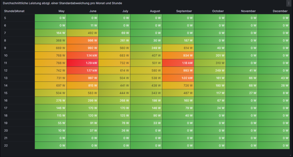
Heatmap of the Hourly and Daily Power Generation
For this, we use the plug-in Grafana visualization Hourly heatmap. We select the according database, and our MySQL query is very simple:
SELECT UNIX_TIMESTAMP(zeitstempel) AS time, ROUND(leistung/1000) AS power FROM anlage;This time, there is also no need for any transformation, but again, we should adjust some panel options in order to beautify our graph, and these are:
- Hourly heatmap → From: Set to 05:00
- Hourly heatmap → To: Set to 23:00
- Hourly heatmap → Group by: Select 60 minutes
- Hourly heatmap → Calculation: Select Mean
- Hourly heatmap → Color palette: Select Spectral
- Hourly heatmap → Invert color palette: (enabled)
- Legend → Gradient quality: Select Low (it already computes long enough in Low mode)
- Standard options → Unit: Select Watt (W)
Then, ideally, after some seconds, you should see something like this:

This visualization is time-consuming. Keep in mind that if you have large amounts of data, it might take several seconds until the graph build up. The Hourly Heatmap is also more detailed than the previous visualizations, and we can point with the mouse pointer on a certain rectangle and get to know the average power on this day and in this hour (if the database has at least one power value per hour). It even shows fluctuations occurring in one day only which might go unnoticed in the previous visualizations. We can realize, for example, that the lower average power which was generated in July this year was not because the sky is greyer in July than in other months, but that there were a few 2…3 days periods with clouded sky where the electricity generation dropped while other days were just perfectly sunny as in June or August. We can also see how the daylight hours dramatically decrease when we reach November.
Daily Energy Generation, split into Time Ranges
The next graph shall visualize the daily energy generation of the solar system over the time, and we split the day into 4 time ranges (morning, lunch, afternoon, evening). The 4 time ranges are not equally large, so you have to pay close attention to the description of the time range. Of course, you can easily change the MySQL query and adapt the time ranges to your own needs. We use the built-in Grafana visualization Time Series. We select the according database, and our MySQL query uses the timestamp and the energy values of the dataset. We also use the uid as we calculate the differences in the (ever increasing) energy value between two consecutive value sets in the dataset.
SELECT DATE(past.zeitstempel) AS time,
       CASE
         WHEN (HOUR(past.zeitstempel)<11) THEN '05:00-11:00'
         WHEN (HOUR(past.zeitstempel)>=11) AND (HOUR(past.zeitstempel)<14) THEN '11:00-14:00'
         WHEN (HOUR(past.zeitstempel)>=14) AND (HOUR(past.zeitstempel)<17) THEN '14:00-17:00'
         WHEN (HOUR(past.zeitstempel)>=17) THEN '17:00-22:00'
       END AS metric,
       SUM(IF(present.energie>=past.energie,IF((present.energie-past.energie<4000),(present.energie-past.energie),NULL),NULL)) AS value
FROM anlage AS present INNER JOIN anlage AS past ON present.uid=past.uid+1
GROUP BY time,metric;
In order to better understand the MySQL query, here are some explanations:
- We determine the time ranges in the form of a CASE statement in which we determine our time ranges and what shall be the textual output for a certain time range.
- We sum up the differences between consecutive energy values in the database over the respective time ranges. This is the task of the SUM operator.
- There might be missing energy values in the dataset, maybe because of network outages or (temporary) issues in the MySQL socket. The IF clauses inside the SUM operator help us to determine if the result of (present.energie-past.energie) would be negative (in case that present.energie is NULL) or if we have an unrealistic value (≥4000) because past.energie is NULL. Such values will be skipped in the calculation.
- We consult the same tables (anlage) two times, one time named as present and one time named as past whereby past the dataset immediately before present is.
- Keep in mind that as time we use the value of past.zeitstempel so that we include the last value that still fits into the time range (although for the calculation of the energy difference, present.zeitstempel would already be the next hour value, e.g.: (past.zeitstempel=16:45 and present.zeitstempel=17:00).
We furthermore should adjust some panel options in order to beautify our graph, and these are:
- Graph styles → Fill opacity: Set to 45%
- Graph styles → Stack Series: Select Normal
- Standard options → Unit: Select Watt-hour (Wh)
- Standard options → Min: Set to 0
- Standard options → Decimals: Set to 0
- Standard options → Color scheme: Select to Classic palette
On the left side, just above the code window, we have to switch from Table to Time Series:
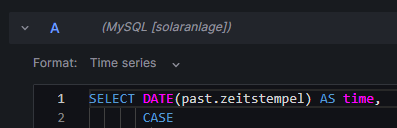
The graph should now look like this:
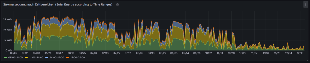
There is one interesting characteristic of the built-in Grafana visualization Time Series which we make use of. If we edit the graph and select the Table view, we will see that Grafana automatically has created a matrix from the results of our MySQL query.
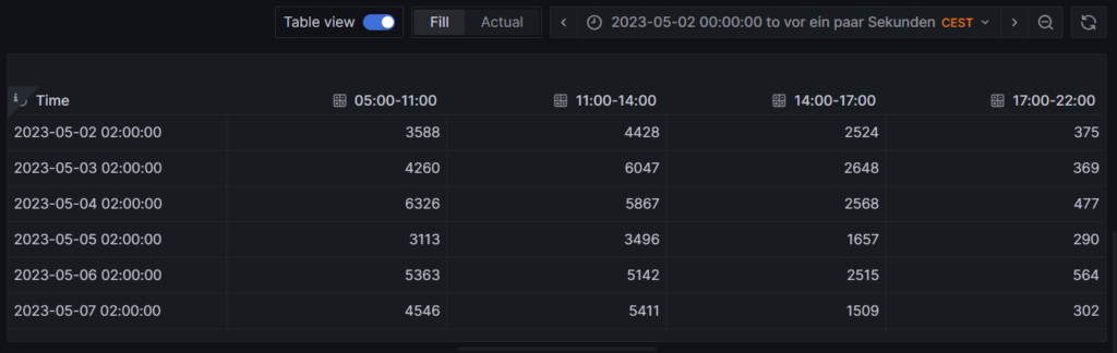
This is astonishing because the MySQL query does not create the matrix itself, but rather delivers an output like:
MariaDB [solaranlage]> SELECT DATE(past.zeitstempel) AS time,
    ->        CASE
    ->          WHEN (HOUR(past.zeitstempel)<11) THEN '05:00-11:00'
    ->          WHEN (HOUR(past.zeitstempel)>=11) AND (HOUR(past.zeitstempel)<14) THEN '11:00-14:00'
    ->          WHEN (HOUR(past.zeitstempel)>=14) AND (HOUR(past.zeitstempel)<17) THEN '14:00-17:00'
    ->          WHEN (HOUR(past.zeitstempel)>=17) THEN '17:00-22:00'
    ->        END AS metric,
    ->        SUM(IF(present.energie>=past.energie,IF((present.energie-past.energie<4000),(present.energie-past.energie),NULL),NULL)) AS value
    -> FROM anlage AS present INNER JOIN anlage AS past ON present.uid=past.uid+1
    -> GROUP BY time,metric
    -> LIMIT 15;
+------------+-------------+-------+
| time       | metric      | value |
+------------+-------------+-------+
| 2023-05-02 | 05:00-11:00 |  3588 |
| 2023-05-02 | 11:00-14:00 |  4428 |
| 2023-05-02 | 14:00-17:00 |  2524 |
| 2023-05-02 | 17:00-22:00 |   375 |
| 2023-05-03 | 05:00-11:00 |  4260 |
| 2023-05-03 | 11:00-14:00 |  6047 |
| 2023-05-03 | 14:00-17:00 |  2648 |
| 2023-05-03 | 17:00-22:00 |   369 |
| 2023-05-04 | 05:00-11:00 |  6326 |
| 2023-05-04 | 11:00-14:00 |  5867 |
| 2023-05-04 | 14:00-17:00 |  2568 |
| 2023-05-04 | 17:00-22:00 |   477 |
| 2023-05-05 | 05:00-11:00 |  3113 |
| 2023-05-05 | 11:00-14:00 |  3496 |
| 2023-05-05 | 14:00-17:00 |  1657 |
+------------+-------------+-------+
15 rows in set (0,197 sec)
I found out that this only works if metric is not a numerical value. For numerical values, the matrix would not be auto generated, the graph would not work like this. Maybe, an additional transformation in Grafana might then be necessary.
Detailed Examinations of the Dataset
Let us look closer to subsets of the dataset and visualize them, in order to get a better understanding of how the solar power generation behaves in reality at selected times.
Power Distribution between 12:00 and 13:00 (4 values per day)
For this, we use the built-in Grafana visualization Heatmap. We select the according database, and our MySQL query is:
SELECT zeitstempel AS time, ROUND(leistung/1000) AS 'Power' FROM anlage
WHERE (HOUR(zeitstempel)=12);
Keep in mind that in my dataset, I register 4 samples per hour in the database. This is defined by the frequency of how often the script described in [1] is executed, and this itself is defined in crontab. You can also have the script be executed every minute, and hence you will register 60 samples per hour in the database which will be more precise but put higher load on your server and on the evaluation of the data in MySQL queries. So, in my case, in the time frame [12:00-13:00], we consider 4 power values, and we filter for these power values simply by looking at timestamps with the value “12” as the hour part. The Heatmap will give the distribution of these 4 power values per day. We must furthermore adjust some panel options, and these are:
- Heatmap → X Bucket: Select Size and set to 24h
- Heatmap → Y Bucket: Select Size and set to Auto
- Heatmap → Y Bucket Scale: Select Linear
- Y Axis → Unit: Select Watt (W)
- Y Axis → Decimals: Set to 1
- Y Axis → Min value: Set to 0
- Colors → Mode: Select Scheme
- Colors → Scheme: Select Oranges
- Colors → Steps: Set to 64

With this Heatmap, we can immediately understand an important detail, and that is: If someone had the assumption that between [12:00-13:00], we generate a lot of power every day in summer, this would clearly be very wrong. In fact, we can recognize that the power generation varies from low to high values on many days. The reason is that even in summer, there are many cloudy days in the location where this solar power generator is located. This might not be true for a different location, and if we had data from Southern Europe (Portugal, Spain, Italy), this might look very different.
Average Power [12:00-13:00]
Now, we shall look at the average power generation between [12:00-13:00] over the year, using the 4 power values that we have register in this time interval every day. For this, we use the built-in Grafana visualization Time Series. We select the according database, and we use two MySQL queries (A and B). Both curves will then be visualized in the diagram with different colors. Our query A calculates the average value per day in the time interval [12:00-13:00] and is displayed in green color:
SELECT zeitstempel AS time, ROUND(AVG(leistung)/1000) AS 'Power [12:00-13:00]' FROM anlage
WHERE (HOUR(zeitstempel)=12)
GROUP BY DATE(zeitstempel);
Our query B takes a 7d average of the average values per day, it therefore is kind of a trend line of the curve we have generated with query A and is displayed in yellow color:
SELECT zeitstempel AS time, (SELECT ROUND(AVG(leistung)/1000) FROM anlage WHERE (HOUR(zeitstempel)=12) AND zeitstempel<=time AND zeitstempel>DATE_ADD(time,INTERVAL-7 DAY)) AS 'Power [12:00-13:00; 7d average]' FROM anlage
WHERE (DATE(zeitstempel)>='2023-05-09')
GROUP BY DATE(zeitstempel);
This graph visualizes the same finding as the previous heatmap. In my opinion, it even shows in a more dramatic way that the average power between [12:00-13:00] even during summer can vary dramatically, and that we simply cannot assume that there is a certain minimum power “guaranteed” in a certain time frame during summer. We also see that in winter, the power generation is minimal, and there is no chance that the solar power generator can contribute to the electricity demand of the home in any meaningful way.
Average Power [12:00-13:00] (calculated as difference of energy values)
One might argue that 4 sampling values per hour are not enough, maybe we were just unlucky and there were clouds in the sky exactly when we were sampling the data. Let us therefore repeat the graph from above, not by using the average of the 4 samples per hour but let us divide the increase of the overall generated energy in the time frame [12:00-13:00] as the base for the power calculation. Again, we will do two queries (A and B) whereby query A is the value on the daily basis:
SELECT present.zeitstempel AS time, (present.energie-past.energie) AS 'Power [12:00-13:00]'
FROM anlage AS present INNER JOIN anlage AS past ON present.uid=past.uid+4
WHERE (TIME_FORMAT(present.zeitstempel,'%H:%i')='13:00');
and where query B shows the 7d average of the daily values:
SELECT zeitstempel AS time, (SELECT AVG(present.energie-past.energie) FROM anlage AS present INNER JOIN anlage AS past ON present.uid=past.uid+4 WHERE (TIME_FORMAT(present.zeitstempel,'%H:%i')='13:00') AND present.zeitstempel<=time AND present.zeitstempel>DATE_ADD(time,INTERVAL-7 DAY)) AS 'Power [12:00-13:00; 7d average]' FROM anlage
WHERE (DATE(zeitstempel)>='2023-05-09')
GROUP BY DATE(zeitstempel);
While we can identify some differences in the green curve between this graph and the previous one, the yellow curve is almost identical. In general, the calculation via the energy values is the more precise one; 4 sample values simply do not seem to suffice as we can see in the differences of the green curves.
The overall conclusion of this curve is the same as in the previous one, however: There are many days where the average power generation between [12:00-13:00] stays well below the expected (larger) values.
Average Hourly Power Generation [June]
The following visualization, again using the built-in Grafana visualization Time Series, shows how the average value of power generated per hour in the month of June varies if we look at the first half and the second half of June. This visualization uses three queries. Query A shows the average power generation of the whole month of June:
SELECT zeitstempel AS time, ROUND(AVG(leistung)/1000) AS 'Power [June 2023]' FROM anlage
WHERE (zeitstempel>'2023-06-01') AND (zeitstempel<'2023-07-01')
GROUP BY HOUR(zeitstempel);
Query B looks at the average power generation of the first half of June:
SELECT zeitstempel AS time, ROUND(AVG(leistung)/1000) AS 'Power [June 2023; first half]' FROM anlage
WHERE (zeitstempel>'2023-06-01') AND (zeitstempel<'2023-06-16')
GROUP BY HOUR(zeitstempel);
Query C looks at the average power generation of the second half of June
SELECT DATE_ADD(zeitstempel, INTERVAL -15 DAY) AS time, ROUND(AVG(leistung)/1000) AS 'Power [June 2023; second half]' FROM anlage
WHERE (zeitstempel>'2023-06-16') AND (zeitstempel<'2023-07-01')
GROUP BY HOUR(zeitstempel);
As time period for the visualization, we select 2023-06-01 00:00:00 to 2023-06-01 23:59:59. You might wonder why we only select one day for the visualization when we examine a whole month. But as we calculate the average value over the full month (indicated in the WHERE clause of the MySQL query), we will receive only data for one day:
MariaDB [solaranlage]> SELECT zeitstempel AS time, ROUND(AVG(leistung)/1000) AS 'Power [June 2023]' FROM anlage
    -> WHERE (zeitstempel>'2023-06-01') AND (zeitstempel<'2023-07-01')
    -> GROUP BY HOUR(zeitstempel);
+---------------------+-------------------+
| time                | Power [June 2023] |
+---------------------+-------------------+
| 2023-06-01 05:00:07 |                 9 |
| 2023-06-01 06:00:08 |               220 |
| 2023-06-01 07:00:07 |               827 |
| 2023-06-01 08:00:07 |              1346 |
| 2023-06-01 09:00:07 |              1530 |
| 2023-06-01 10:00:07 |              1711 |
| 2023-06-01 11:00:07 |              1814 |
| 2023-06-01 12:00:08 |              1689 |
| 2023-06-01 13:00:07 |              1512 |
| 2023-06-01 14:00:08 |              1215 |
| 2023-06-01 15:00:07 |               853 |
| 2023-06-01 16:00:07 |               458 |
| 2023-06-01 17:00:07 |               264 |
| 2023-06-01 18:00:07 |               192 |
| 2023-06-01 19:00:07 |               133 |
| 2023-06-01 20:00:07 |                59 |
| 2023-06-01 21:00:07 |                 9 |
| 2023-06-01 22:00:07 |                 0 |
+---------------------+-------------------+
18 rows in set (0,035 sec)
This also explains the sequence DATE_ADD(zeitstempel, INTERVAL -15 DAY) in query C. That sequence simply “brings back” the result curves from the day 2023-06-16 to the day 2023-06-01 and thus into our selected time period.
We also need to adjust some panel options, and these are:
- Standard options → Unit: Select Watt (W)
- Standard options → Min: Set to 0
- Standard options → Max: Set to 2500
- Standard options → Decimals: Set to 1
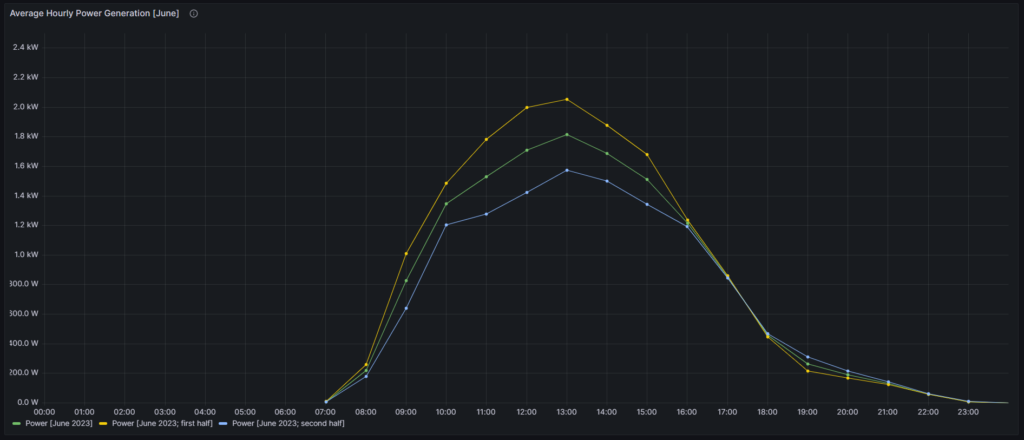
The green curve displays the average data over the whole month of June whereas the yellow curve represents the first half, and the blue curve represents the second half. We can see that this year (2023), the second half of June was much worse than the first half of June, in terms of power generation. Only in the time window [16:00-18:00], all three curves show the same values.
Power Distribution between 12:00 and 13:00 [June 2023]
Let us go back to the assumption we used for the second visualization on this article where we assumed a normal distribution of power values for a reasonably small timeframe (one hour over one month). Is this actually a true or maybe a wrong assumption? In order to get a better feeling, we use the built-in Grafana visualization Histogram and look how the power value samples (4 per hour) distribute in the month of June, in the first half of June (where we had a sunny sky), and in the second half of June (where we had a partially cloudy sky).
For the following three histograms, we use the panel options:
- Histogram → Bucket size: Set to 50
- Histogram → Bucket offset : Set to 0
- Standard options → Unit: Select Watt (W)
- Standard options → Min: Set to 0
- Standard options → Max: Set to 2500
- Standard options → Color scheme: Select Single color
The first histogram shows the distribution of power samples (120 in total) over the whole month of June:
SELECT zeitstempel, ROUND(leistung/1000) AS 'Power 12:00-13:00 [June 2023]' FROM anlage
WHERE (zeitstempel>'2023-06-01') AND (zeitstempel<'2023-07-01')
  AND (HOUR(zeitstempel)=12);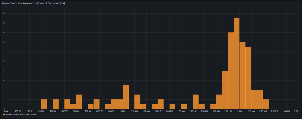
The second histogram shows the distribution of power samples (60 in total) over the first half of June:
SELECT zeitstempel, ROUND(leistung/1000) AS 'Power 12:00-13:00 [June 2023; first half]' FROM anlage
WHERE (zeitstempel>'2023-06-01') AND (zeitstempel<'2023-06-16')
  AND (HOUR(zeitstempel)=12);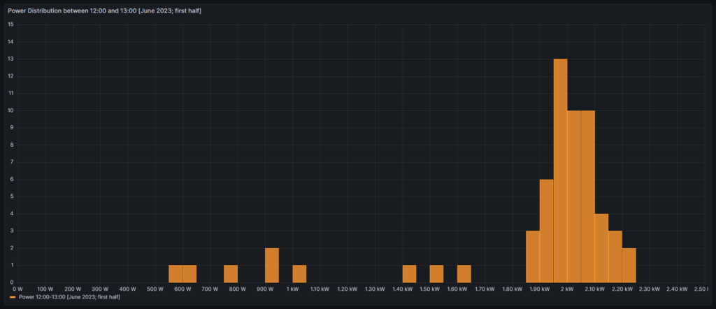
The third histogram shows the distribution of power samples (60 in total) over the second half of June:
SELECT zeitstempel, ROUND(leistung/1000) AS 'Power 12:00-13:00 [June 2023; second half]' FROM anlage
WHERE (zeitstempel>'2023-06-16') AND (zeitstempel<'2023-07-01')
  AND (HOUR(zeitstempel)=12);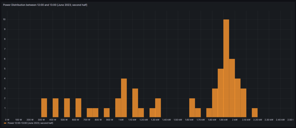
From all curves, we can see that the distribution that we see is by no means a normal distribution. It certainly has a region where we have a bell-shaped density of power values, but during periods with cloudy skies, we can also have many values in the range below the bell-shaped values of the solar generator. Therefore, the assumption of a normal distribution does not hold true in reality.
Conclusion
Visualizations
Grafana allows us to create advanced visualizations from MySQL data with little effort. The point with some less used visualizations in Grafana however, is that there is little documentation available, or to say it in a different way: Sometimes the documentation is sufficient if you already know how it works, but insufficient if you do not yet know how it works. I hope that at least with this article, I could contribute to enlarge knowledge.
Solar Power Generation
The data used in this example shows a solar power generation unit in Germany, facing the East. From the visualized data, we can draw several conclusions:
- Peak power of the installed solar power system is shortly before lunch time and decreases already significantly after 14:00.
- While power generation looks good until even October, from November on, the yield is poor.
- While the generated electricity in the winter months might still help to decrease the electricity bill, it becomes clear that if you were to use a heat pump for the heating of your home, you cannot count on solar power generation to support you in a meaningful way until you have some 50 kW+ peak solar capacity on a large roof.
- As the solar power generation peaks shortly before noon, it might make sense to combine units that face to the East and units that face to the West. This observation is in-line with recent proposals that claim that units facing South are not much better than a combination of units facing East and West (e.g., [3]).
Outlook
The visualizations given here are only an easy beginning. We might want to use more serious statistical analysis to answer questions like:
- Can we infer from a bad start in the morning (little power) that the rest of the day will stay like this?
- How probable is it that we have 3+ cloudy days (with little electricity) in a row, and that translates to: If it rained today, should I wait for 1…3 more days before I turn on the washing machine?
- Does it make economic sense to invest in a battery storage in order to capture excess electricity in summer days? How large should this battery be?
Files
The following dataset was used for the graphs:
Sources
- [1] = Smarthome: AVM-Steckdosen per Skript auslesen – Gabriel Rüeck (caipirinha.spdns.org)
- [2] = Download Grafana | Grafana Labs
- [3] = Ost-West-Ausrichtung von Photovoltaikanlagen (solarenergie.de)
Disclaimer
- Program codes and examples are for demonstration purposes only.
- Program codes are not recommended be used in production environments without further enhancements in terms of speed, failure-tolerance or cyber-security.
- While program codes have been tested, they might still contain errors.
Smarthome: AVM-Steckdosen per Skript auslesen
Zusammenfassung
In diesem Artikel stelle ich ein bash-Skript vor, mit welchem man Smart-Home-Daten der Steckdosen FRITZ!DECT 200 oder FRITZ!DECT 210 aus einer FRITZ!Box der Firma AVM auslesen kann. Ein weiteres Skript bedient sich des ersten Skripts und speichert Daten in einer einfachen MySQL-Datenbank.
Voraussetzungen
- Es wird eine der neueren FRITZ!Boxen der Firma AVM mit aktueller Firmware eingesetzt. Eine 7490 ist zählt bereits als eine der “neueren” Boxen; insofern stehen die Chancen gut, dass viele Interessenten dieses Skript einsetzen können.
- Es werden eine oder mehrere der AVM-Steckdosen FRITZ!DECT 200 oder FRITZ!DECT 210 eingesetzt. Mit diesen ist das Skript erfolgreich getestet worden.
- Getestet wurde mit einer schon älteren FRITZ!Box 7490 und der Firmware 7.57.
- Idealerweise hat man einen dauerhaft laufenden kleinen Linux-Server, auf dem die hier gezeigten Skripte und die MySQL-Datenbank laufen können.
Beschreibung und Nutzung
Die beiden AVM-Steckdosen FRITZ!DECT 200 oder FRITZ!DECT 210 sind, in Verbindung mit einer der neueren FRITZ!-Boxen, eine sehr gute Möglichkeit zur Steuerung von Strom-Verbrauchen und -Erzeugern und zur Leistungs-, Energie- und Temperaturmessung. Die Steckdosen messen dabei die durchfließende Leistung unabhängig von der Richtung und können daher auch sehr gut zur Erfassung der Stromerzeugung bei Balkon-Kraftwerken benutzt werden.
Wenn die FRITZ!Box konfiguriert wird, legt sie einen Standardbenutzer fritzxxxx an, sofern man den Login mit lediglich einem Passwort aus dem Heimnetzwerk erlaubt hat. In der FRITZ!Box findet man diesen Benutzer auf der Seite System → FRITZ!Box-Benutzer. Dieser Benutzer sollte für unsere Zwecke die Rechte Smart Home haben. Bei mir sieht das so aus:

Die üder das Protokoll DECT verbundenen Smarthome-Geräte findet man in der FRITZ!-Box auf der Seite Smart Home → Geräte und Gruppen.
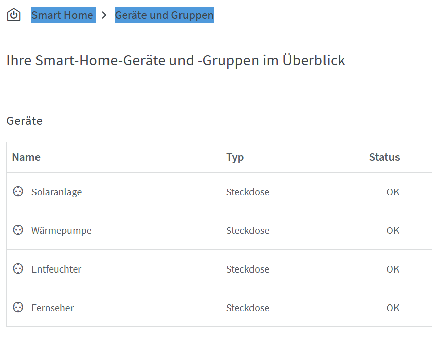
Klickt man auf ein Gerät, so findet man in den Konfigurationseinstellungen, dann findet man die Aktor Identifikationsnummer (AIN) des entsprechenden Geräts. Diese wird für das Skript benötigt. Man beachte, dass es sich um zwei Zahlenblöcke handelt, die durch genau ein Leerzeichen getrennt sind.
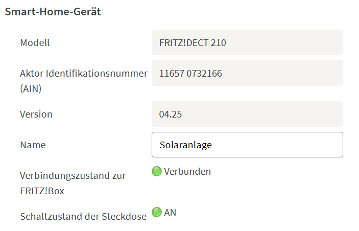
Im folgenden Skript sind die AINs meiner vier Steckdosen mit den bei diesen Modellen möglichen Abfragen für Leistung, Energie, Temperatur und Spannung eingetragen. Das Skript basiert auf einer Vorlage aus [1], die aber nach einem Firmware-Update nicht mehr richtig funktionierte, weswegen ich Änderungen durchgeführt habe. Dabei habe ich mich an der technischen Dokumentation aus [2], [3] orientiert. Man muss natürlich noch die IP-Adresse seiner FRITZ!-Box (hier mit 192.168.2.8 angenommen), den Benutzernamen (USER) und das Passwort (PASS) anpassen.
Der erste Teil des Skripts erzeugt eine gültige Session ID, die man im Verlauf der eigentlichen Abfrage benötigt. Das Vorgehen dazu ist in [2] beschrieben; im Wesentlichen müssen Zeichenfolgen ausgewertet werden, zwischendrin muss mal auf UTF-16LE-Codierung gewechselt werden, und es müssen auch noch der Benutzername und das Passwort übermittelt werden.
Im zweiten Teil nutzen wir die Session ID und fragen eines der vier Geräte und eines der vier möglichen Argumente ab. Aufgerufen wird das Skript (es heißt bei mir “avm_smartsocket.sh”) mit:
./avm_smartsocket.sh Fernseher|Solaranlage|Wärmepumpe|Entfeuchter energy|power|temperature|voltageIch denk, durch die klare Struktur lässt sich das Skript auch sehr leicht für eigene Zwecke anpassen.
#!/bin/bash
#
# https://raspberrypiandstuff.wordpress.com/2017/08/03/reading-the-temperature-from-fritzdect-devices/
# modified by Gabriel Rüeck, 2023-12-06
#
# -----------
# definitions
# -----------
readonly TERM_LRED='\e[91m'
readonly TERM_RESET='\e[0m'
readonly FBF="http://192.168.2.8"
readonly USER="fritz1234"
readonly PASS="geheimes_fritzbox_passwort"
# -------------------
# check for arguments
# -------------------
if [ $# -lt 2 ]; then
   echo -e "${TERM_LRED}Call the function with ${0} Fernseher|Solaranlage|Wärmepumpe|Entfeuchter energy|power|temperature|voltage.${TERM_RESET}\n"
   exit 1
fi
# ---------------
# fetch challenge
# ---------------
CHALLENGE=$(curl -s "${FBF}/login_sid.lua" | grep -Po '(?<=<Challenge>).*(?=</Challenge>)')
# -----
# login
# -----
MD5=$(echo -n ${CHALLENGE}"-"${PASS} | iconv -f UTF-8 -t UTF-16LE | md5sum -b | awk '{print substr($0,1,32)}')
RESPONSE="${CHALLENGE}-${MD5}"
SID=$(curl -i -s -k -d "response=${RESPONSE}&username=${USER}" "${FBF}/login_sid.lua" | sed -n 's/.*<SID>\([[:xdigit:]]\+\)<\/SID>.*/\1/p')
# ----------
# define AIN
# ----------
case "${1}" in
  Fernseher)        AIN="11630%200239598";;
  Solaranlage)      AIN="11657%200732166";;
  Wärmepumpe)       AIN="11630%200325768";;
  Entfeuchter)      AIN="11630%200325773";;
  *)                exit 1;;
esac
# ------------
# fetch values
# ------------
case "${2}" in
  energy)       RESULT=$(curl -s ${FBF}'/webservices/homeautoswitch.lua?ain='${AIN}'&sid='${SID}'&switchcmd=getswitchenergy');;
  power)        RESULT=$(curl -s ${FBF}'/webservices/homeautoswitch.lua?ain='${AIN}'&sid='${SID}'&switchcmd=getswitchpower');;
  temperature)  RESULT=$(curl -s ${FBF}'/webservices/homeautoswitch.lua?ain='${AIN}'&sid='${SID}'&switchcmd=gettemperature')
                [[ ${RESULT} -lt 0 ]] && RESULT=0;;
  voltage)      RESULT=$((curl -s ${FBF}'/webservices/homeautoswitch.lua?ain='${AIN}'&sid='${SID}'&switchcmd=getdevicelistinfos') |  sed -n 's/.*<voltage>\(.*\)<\/voltage>.*/\1/p');;
  *)            exit 1;;
esac
# -------------
# output values
# -------------
echo ${RESULT}
Wichtig ist noch wissen, welche Werte wir jeweils erhalten, und das sind bei den AVM-Steckdosen FRITZ!DECT 200 oder FRITZ!DECT 210:
| Argument | Angezeigtes Resultat |
| power | Momentane Leistung in mW |
| energy | Akkumulierte Energiemenge in Wh |
| temperature | Momentane Temperatur in 0,1 °C (Beispiel: 65 ≙ 6,5 °C) |
| voltage | Momentane Netzspannung in mV |
Nun wollen wir mit dem oben gelisteten Skript Daten der Steckdose Solaranlage auslesen und in einer MySQL-Datenbank speichern. Dazu setzen wir eine kleine und sehr einfache Datenbank auf:
# Datenbank für Analysen der Solaranlage
# V1.0; 2023-05-01, Gabriel Rüeck <gabriel@rueeck.de>, <gabriel@caipirinha.spdns.org>
# Create a new database
CREATE DATABASE solaranlage DEFAULT CHARSET utf8mb4 COLLATE utf8mb4_general_ci;
GRANT ALL ON solaranlage.* TO 'gabriel';
USE solaranlage;
SET default_storage_engine=Aria;

CREATE TABLE anlage          (zeitstempel    TIMESTAMP NOT NULL DEFAULT CURRENT_TIMESTAMP,\
                              leistung       INT UNSIGNED DEFAULT NULL,\
                              energie        INT UNSIGNED DEFAULT NULL);
Zugegebenermaßen ist das CHARSET der Datenbank ziemlich egal; man hätte nicht unbedingt noch utf8mb4 vorsehen müssen. Ich setze das aber generell für meine Datenbanken, nachdem ich mal längere Zeit nach einem Fehler in einer komplexeren Datenbank gesucht hatte und dann lernen musste, dass UTF-8 bei MySQL nicht automatisch alle UTF-8-Zeichen beinhaltet [4].
Der Zeitstempel muss beim Beschreiben der Datenbank nicht explizit gesetzt werden; per Default wird der momentane Zeitstempel des Datenbank-Servers benutzt.
Das nun folgende Skript nutzt unser erstes Skript, liest Daten für Leistung und Energie aus und speichert sie in der MySQL-Datenbank:
#!/bin/bash
#
# Dieses Skript liest die Leistung und die erzeugte Energiemenge der Solaranlage und speichert das Ergebnis in einer MySQL-Datenbank ab.
#
# V1.0; 2023-05-01, Gabriel Rüeck <gabriel@rueeck.de>, <gabriel@caipirinha.spdns.org>
#
# CONSTANTS
declare -r    MYSQL_DATABASE='solaranlage'
declare -r    MYSQL_SERVER='localhost'
declare -r    MYSQL_USER='gabriel'
declare -r    MYSQL_PASS='geheimes_mysql_passwort'
declare -r    READ_SCRIPT='~/avm_smartsocket.sh'

# VARIABLES
declare -i power energy

# PROGRAM
power=$(${READ_SCRIPT} Solaranlage power)
energy=$(${READ_SCRIPT} Solaranlage energy)
mysql --default-character-set=utf8mb4 -B -N -r -D "${MYSQL_DATABASE}" -h ${MYSQL_SERVER} -u ${MYSQL_USER} -p ${MYSQL_PASS} -e "INSERT INTO anlage (leistung,energie) VALUES (${power},${energy});"
Abhängig davon, wie oft man dieses Skript laufen lässt und Daten abspeichern lässt, ergeben sich dann im folgenden Beispiel genannten Einträge in der Datenbank:
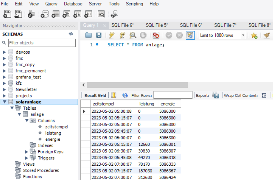
Diese Daten können dann in anderen Systemen ausgewertet und visualisiert werden.
Zusammenfassung
In diesem einfachen Beispiel sieht man, wie man Smart-Home-Daten der Steckdosen Fritz!DECT 200 oder Fritz!DECT 210 aus einer FRITZ!-Box der Firma AVM abfragen und sich die Daten in einer MySQL-Datenbank zur weiteren Verwendung speichern kann. Sicherlich lässt sich dieses Prinzip auch auf Smart-Home-Geräte anderer Hersteller anwenden, sofern deren Schnittstellen hinreichend offen und beschrieben sind.
Quellenangaben
- [1] = Reading the temperature from FRITZ!DECT devices – Raspberry Pi and Stuff (wordpress.com)
- [2] = Session-IDs im FRITZ!Box Webinterface
- [3] = AHA-HTTP-Interface
- [4] = encoding – What is the difference between utf8mb4 and utf8 charsets in MySQL? – Stack Overflow
Disclaimer
- Der Programmcode und die Beispiele sind lediglich zu Demonstrationszwecken gedacht.
- Der Programmcode wurde nicht auf Geschwindigkeit optimiert (Es ist sowieso ein Bash-Skript, da darf man keine Wunder erwarten.).
- Der Programmcode wurde nicht unter dem Gesichtspunkt der Cybersicherheit geschrieben. Für den Einsatz in Produktivumgebungen müssen möglicherweise Anpassungen vorgenommen werden.
- Der Programmcode wurde zwar getestet, kann aber dennoch Fehler enthalten.