Sensitivity Analysis for Business Cases
Sensitivity Analysis
-
sales price
-
sales numbers
-
material cost
-
development cost
1-Dimensional Sensitivity Analysis
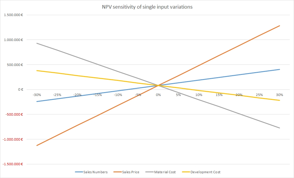
From the graph shown above, we can already get some important insights with respect to our example business case:
- The sales price has the largest influence on the resulting NPV. If sales prices drop by 5% only, our project does not add any more value to the business. Therefore, we must make sure that:
- our estimation of the sales price is as good as possible and not “inflated”
- we develop suitable countermeasures in case the sales price drops in the market
- The sales numbers and the development cost have less influence on the NPV; hence they are not our first concern.
2-Dimensional Sensitivity Analysis
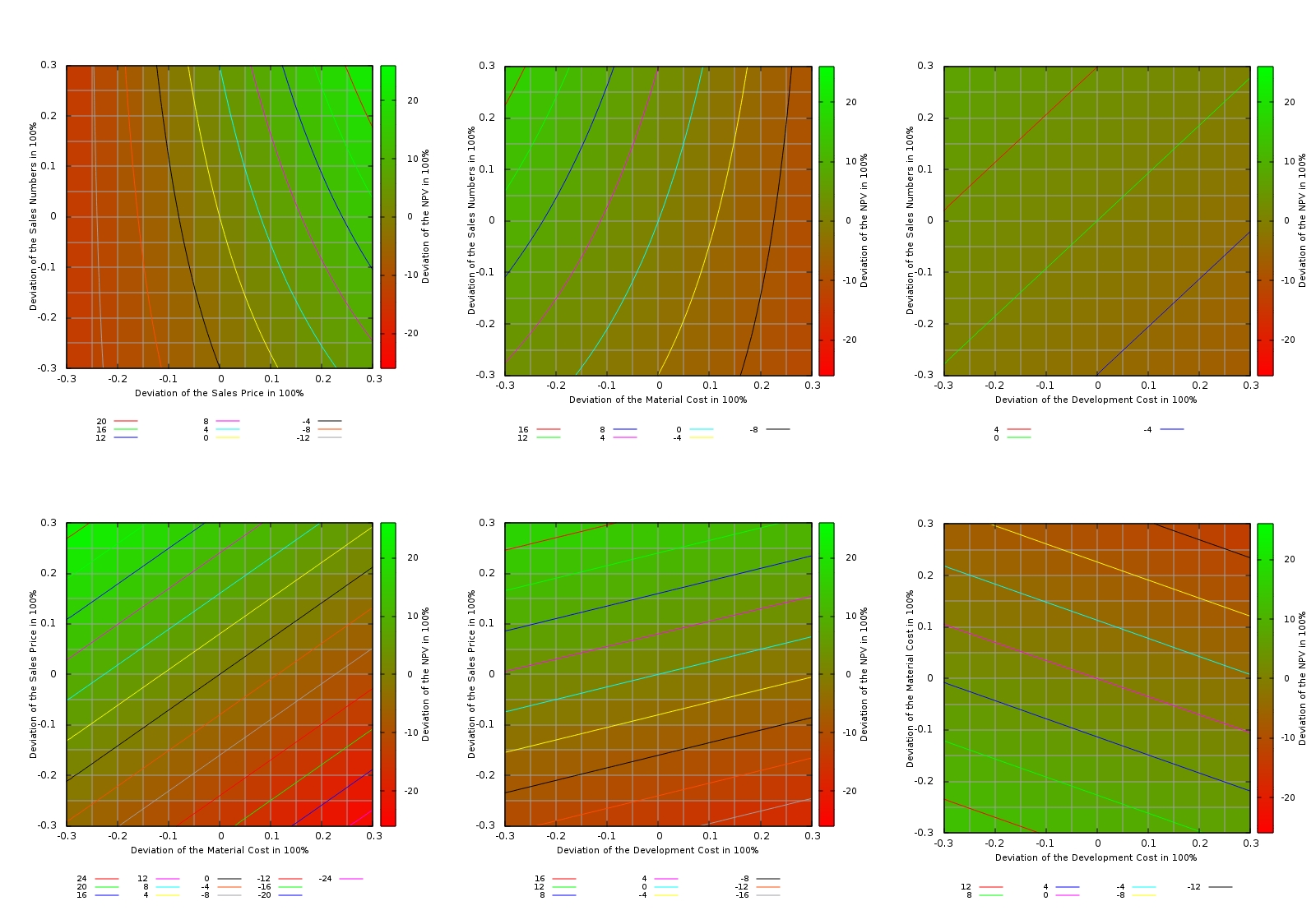
Now, we will change two input variables at a time and leave the others constant (ceteris paribus). The tables for these investigations are listed on the sheet Scenario Analysis (2D). In additional to the overall monetary values of the NPV, the relative increments and decrements in % have been listed in tables on the right side of the respective scenario. I tried to visualize the result in Excel, but I found the related Excel graphics not very adequate. With the open-source tool gnuplot, it is however possible to create meaningful graphs. I am a novice with this tool and certainly, more elaborate visualizations are possible. Nevertheless, for a first interpretation, heat maps and contour lines serve the purpose. In order to create them, I had to transpose the tables into formats as shown on the sheet Scenario Analysis (2D), gnuplot. Furthermore, I had to use the setup commands listed on the sheet Init gnuplot in order to make gnuplot output the graphs below.
The graphs show heat maps with contour lines, and I believe that this is a good visualization for a 2-D sensitivity analysis although initially, it might take a while to familiarize yourself with this kind of visualization. The areas with green colour represent areas in which the NPV is better than in our base estimation, the areas with red colour represent areas in which the NPV is worse than in our initial base estimation. Each graph also has a contour lines which is labeled “0” in the legend, and this contour line represents combinations of the input variables where the NPV is the same than in our base estimation.
From the tables on the sheet Scenario Analysis (2D) and the graphs, we can get additional insight which is not accessible in the 1-D sensitivity analysis. We can draw the following conclusions, for example:
- If an increase in the sales price leads to a drop of the sales numbers of less than 15%, we still get a higher NPV than in our base estimation. If the price elasticity of our product warrants that move, then we should definitively go for it!
- If the development of additional features can yield a 10% increase of the sales price, we can easily spend 30% more development budget on those features.
- We can easily spend 25% more development budget if that additional development effort results in a 10% lower material cost.
3-Dimensional Sensitivity Analysis
I expect that with virtual reality gear like Oculus Rift, we might very soon be able to move ahead and create a visualization like a room that is filled with a coloured gas. By moving through that room and moving you head in the vertical, you might be able to explore that room in three dimensions. Similarly to the added insight that we gained while moving from a 1-D sensitivity analysis to a 2-D sensitivity analysis, we might find yet more additional insight.
Outlook
Clearly, heat maps with contour lines offer valuable insight in business cases, especially if we limit the heat maps to visualizations of those input variables that have proven to have the largest impact in the 1-D sensitivity analysis. In our business case example, the underlying formula for the NPV is simple which is reflected in the slightly curved or straight contour lines of the graphs. In more complicated business cases or in different applications, we might expect different and non-linear behaviours that then would result in more complicated heat maps and contour lines. We might find, for example that there can be a local minimum (a red-coloured spot) in our heat map which would then mean that we have a found a combination of our input variables that we must avoid under all circumstances, similar to a cliff in the ocean where we have to ship around. This would be visible immediately in the heat map. However, mathematically, we can even find such “cliffs” in an n-dimensional sensitivity analysis using multi-variable calculus although we are not able to “visualize” that in our mind. Such approaches might delivers us insight into dangerous or unfortunate combinations of input variables that other methods might not offer.

